Introduction to Population Genetics

Chapter 18 - Introduction to Genetic Analysis (12th ed.)

Peter Sørensen

Center for Quantitative Genetics and Genomics

Aarhus University

2026-03-27

Why Study Population Genetics?

• Assess genetic disease risk
  
• Evaluate how breeding practices affect genetic diversity
  
• Understand risks of inbreeding in small or fragmented populations
  
• Explore relationships among human populations
  
• Study genomic adaptation to different environments
  
• Explain how populations and species evolve

Population genetics addresses questions with clear societal relevance.

It provides tools to assess genetic disease risk and to evaluate how breeding practices influence genetic diversity.

It helps determine whether small or fragmented populations are vulnerable to inbreeding and loss of variation.

Beyond applied questions, it also addresses fundamental evolutionary issues.

How are human populations related? How have genomes adapted to different environments? And how do allele frequencies change over time?

In essence, population genetics connects molecular variation to practical applications and to the mechanisms that drive evolutionary change.

What Is Population Genetics?

Population genetics explains how evolutionary processes shape patterns of genetic variation and their consequences.

Patterns

• DNA variation
  
• Allele frequencies
  
• Linkage disequilibrium
  
• Population differences

→

Processes

• Mutation
  
• Migration
  
• Recombination
  
• Genetic drift
  
• Natural selection

→

Consequences

• Adaptation
  
• Disease risk
  
• Population history
  
• Conservation genetics

Population genetics tries to answer a simple question:

Why does genetic variation look the way it does?

Across genomes we observe patterns. We see differences in DNA sequences, allele frequencies, linkage disequilibrium, and genetic diversity across populations.

These are measurable patterns in genetic data.

But patterns alone do not explain themselves.

Population genetics tries to understand the processes that generate those patterns.

Five fundamental evolutionary forces shape genetic variation:

mutation introduces new alleles, migration moves alleles between populations, recombination reshuffles alleles into new haplotypes, genetic drift causes random fluctuations in finite populations, and natural selection changes allele frequencies when some genotypes leave more offspring than others.

These processes determine how allele frequencies change across generations.

Finally, these evolutionary processes have important consequences.

They influence adaptation, disease risk, population history, and many practical applications in medicine, conservation biology, and forensics.

So the goal of population genetics is to connect:

observable patterns → evolutionary processes → biological consequences.

Everything we cover in this chapter fits into that framework.

Population Genetics

What Is a Population?

• Individuals of the same species
  
• An interbreeding group
  
• A defined sampling unit

A population is defined by gene exchange and a shared contribution to future generations.

What Is Population Genetics?

• Study of genetic variation within populations
  
• Study of changes in allele frequencies over time

Driven by evolutionary forces:

• Mutation
  
• Migration (gene flow)
  
• Recombination
  
• Genetic drift
  
• Natural selection
  
• Mating systems

Focus: how evolutionary forces shape allele frequencies across generations.

First, what is meant by a population?

In biology, it refers to a group of individuals of the same species that interbreed and exchange genes.

In genetics, it also refers to the group from which individuals are sampled to estimate allele frequencies.

Population boundaries are therefore defined by gene exchange and shared reproductive contribution.

What, then, is population genetics?

It is the study of genetic variation within populations and the analysis of how allele frequencies change over time.

The emphasis is not on individual pedigrees, but on the genetic composition of the population as a whole.

Allele frequencies change because of evolutionary forces: mutation introduces new variation, migration moves alleles between populations, recombination reshuffles genetic material, genetic drift causes random fluctuations, natural selection drives systematic change, and mating systems alter genotype structure.

Population genetics seeks to understand how these forces interact to shape genetic variation across generations.

Learning Goals — Population Genetics

1. Detecting Genetic Variation

• Identify major types of DNA variation
  
• Explain locus, allele, haplotype, and phase

2. Gene Pool & Hardy–Weinberg

• Define the gene pool and calculate allele and genotype frequencies
  
• State the Hardy–Weinberg law and its assumptions
  
• Test for equilibrium and explain causes of deviation

3. Mating Systems & Inbreeding

• Distinguish mating systems
  
• Explain effects of nonrandom mating on genotype frequencies
  
• Define inbreeding and describe its genetic consequences

4. Measurement of Genetic Variation

• Understand and interpret common statistics used to quantify genetic variation in populations

5. Evolutionary Forces

• Describe how mutation, migration, recombination, drift, and selection change allele frequencies
  
• Explain population size effects and genetic drift
  
• Distinguish major forms of selection
  
• Explain linkage disequilibrium and its decay
  

This chapter focuses on genetic variation at the population level.

The learning goals are organized into five main areas.

First, detecting genetic variation. This includes identifying major types of DNA variation and understanding key concepts such as locus, allele, haplotype, and phase.

Second, the gene pool and Hardy–Weinberg equilibrium. This involves calculating allele and genotype frequencies, stating the Hardy–Weinberg law and its assumptions, and testing for deviations from equilibrium.

Third, mating systems and inbreeding. This includes understanding how nonrandom mating alters genotype structure and recognizing the genetic consequences of inbreeding.

Fourth, measurement of genetic variation. Here we introduce statistics used to quantify genetic diversity in populations, such as segregating sites, haplotype counts, gene diversity, and nucleotide diversity.
These measures allow us to compare levels of genetic variation across populations and species.

Fifth, evolutionary forces. Mutation, migration, recombination, genetic drift, and natural selection change allele frequencies over time.
This section also includes linkage disequilibrium and its decay.

The overall objective is not only to perform calculations, but to interpret what patterns of genetic variation reveal about evolutionary processes.

The overall objective is not only to perform calculations, but to interpret what patterns of genetic variation reveal about evolutionary processes.

1. Detecting Genetic Variation

DNA Variation in Populations

DNA variation occurs at specific genomic locations

• A locus = a position in the genome
  • A single nucleotide
    
  • Or a longer DNA region

Humans are diploid
→ two alleles at each autosomal locus

At a locus, individuals may carry different alleles.

Major types of genetic variation

• Single nucleotide polymorphisms (SNPs)
  
• Small insertions/deletions (indels)
  
• Repeat-length variants (microsatellites / STRs)
  
• Structural variants (CNVs, inversions)

SNPs

• Single base substitution (A, C, G, or T)
  
• Most abundant variant type
  
• Usually biallelic
  
• Relatively low mutation rate

Microsatellites (STRs)

• Short motifs (2–6 bp) repeated in tandem
  
• Alleles differ in repeat number
  
• Often highly polymorphic
  
• Higher mutation rate

SNPs → abundant and relatively stable
Microsatellites → highly variable

Population genetics examines variation at specific genomic locations, called loci.

A locus is simply a position in the genome. It may refer to a single nucleotide or to a longer DNA region.

Humans are diploid, meaning two copies of each autosomal chromosome are present. At each locus, an individual therefore carries two alleles, one inherited from each parent.

Genetic variation occurs at multiple scales: single-base substitutions, small insertions or deletions, repeat-length variants, and larger structural changes.

The primary focus here is on SNPs and microsatellites.

SNPs are single nucleotide substitutions. They are abundant across the genome, usually biallelic, and mutate at relatively low rates.

Microsatellites consist of short repeated motifs. Alleles differ in the number of repeats. They mutate more rapidly and are often highly polymorphic.

In simple terms, SNPs are abundant and relatively stable, whereas microsatellites are fewer in number but highly variable.

Visualizing Genetic Variation

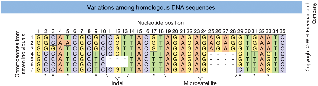
Figure 18-1. Aligned DNA sequences from seven chromosomes. Asterisks indicate SNPs. Indels and a microsatellite region are also shown.

This figure shows aligned DNA sequences from seven different chromosomes.

Each row represents a chromosome from a different individual. Each column represents a nucleotide position.

Notice that most positions are identical across individuals. These are conserved sites.

The asterisks mark single nucleotide polymorphisms, or SNPs. At these positions, at least one individual has a different base.

We also see insertions and deletions — called indels. These occur when a stretch of nucleotides is either missing or inserted in some individuals.

Finally, the figure shows a microsatellite region. This is a short repeated sequence. Different individuals have different numbers of repeats.

The key idea: A locus can exhibit several types of variation — single-base differences, small insertions or deletions, and repeat-length variation.

All of these contribute to genetic diversity in populations.

From DNA to Genotype Data

Genomic technologies allow measurement of variation at thousands to millions of loci.

Marker-based genotyping

• Assay predefined variants
  (SNP arrays, STR panels)
  
• Efficient for large sample sizes

Sequencing-based approaches

• Discover and genotype variants simultaneously
  
• Provide more comprehensive genomic information

Large genotype datasets across many loci form the foundation of population genetic analysis.

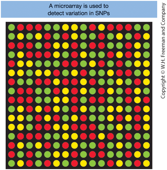
Figure 18-2. Microarray for SNP genotyping

• Each dot = one SNP
  
• Red/green = homozygous
  
• Yellow = heterozygous

Modern genomic technologies allow us to measure variation at thousands to millions of loci across the genome.

There are two main strategies.

Marker-based genotyping assays predefined variants, such as SNP arrays or STR panels. These methods are efficient for large sample sizes, but they only capture known variants.

Sequencing-based approaches directly read DNA sequence. They allow both discovery and genotyping of variants. Sequencing provides richer information, but requires more computational processing.

In both cases, the result is a large genotype matrix: many individuals by many loci. That dataset forms the foundation of population genetic analysis.

The figure shows a SNP microarray. Each dot represents a single SNP. Color indicates genotype — red and green are homozygous, yellow is heterozygous.

Technological advances like this made modern population genetics possible.

The Genotype Matrix

After genotyping, data are organized into an n × m matrix.

• n = number of individuals (rows)
  
• m = number of loci (columns)
  
• Each cell = genotype at one locus for one individual

Common SNP Coding (biallelic loci)

Code	Genotype
0	Homozygous reference
1	Heterozygous
2	Homozygous alternative

	SNP₁	SNP₂	SNP₃	…
Ind₁	0	1	2
Ind₂	1	1	0
Ind₃	2	0	1
…

Biological data → Numerical matrix → Statistical analysis

After genotyping, the data are organized into a matrix.

Each row represents an individual. Each column represents a locus, typically a SNP.

Each entry encodes the genotype at that locus. For biallelic SNPs, numeric coding is commonly used: 0, 1, or 2, representing the number of alternative alleles carried by the individual.

The result is an n by m matrix, with n individuals and m loci.

This structure is fundamental. It converts biological information into a numerical representation suitable for quantitative analysis.

From this matrix, allele frequencies can be calculated. Measures such as heterozygosity and linkage disequilibrium can be derived. Statistical models can then be applied.

The transformation from biological variation to matrix representation is what enables modern population genetics and genomics.

Linked Loci, Haplotypes, and Phase

Loci are arranged along chromosomes.

• Physically close loci recombine less frequently
  
• Nearby alleles tend to be inherited together

These allele combinations on a single chromosome are called haplotypes.

Definition:
A haplotype = a set of alleles at multiple loci
located on the same chromosome copy.

Example: Two linked loci

• Locus 1: A / a
  
• Locus 2: B / b

Possible haplotypes: AB, Ab, aB, ab

Phase

• Genotype: alleles present at loci (unphased)
  
• Haplotype: alleles on one chromosome (phased)

The same genotype can correspond to different phases.

So far we have treated loci as independent.

In reality, loci are arranged along chromosomes. If two loci are physically close, recombination between them is less likely. As a result, nearby alleles tend to be inherited together.

These combinations of alleles on a single chromosome are called haplotypes.

Because humans are diploid, each individual carries two haplotypes for a chromosomal region.

For example, consider two loci: uppercase A or lowercase a at the first locus, and uppercase B or lowercase b at the second locus.

Four haplotypes are possible: uppercase A–uppercase B, uppercase A–lowercase b, lowercase a–uppercase B, and lowercase a–lowercase b.

A genotype tells us which alleles are present at each locus. But it does not tell us which alleles occur together on the same chromosome.

That arrangement is called phase.

For example, an individual with genotype uppercase A–lowercase a and uppercase B–lowercase b could have haplotypes uppercase A–uppercase B and lowercase a–lowercase b, or uppercase A–lowercase b and lowercase a–uppercase B.

These individuals share the same genotype, but differ in phase.

Understanding haplotypes and phase becomes important when studying recombination and linkage disequilibrium.

Inheritance of Haplotypes

Mother

Haplotype 1: A ─── B
Haplotype 2: a ─── b

Father

Haplotype 1: A ─── b
Haplotype 2: a ─── B

Case 1: No Crossover Between A and B

Transmitted haplotypes remain intact.

Example offspring:

A ─── B
a ─── B

Haplotypes: A B / a B
Genotype: A a B B

Case 2: Crossover Between A and B

Recombination creates new haplotypes.

Example recombinant haplotypes:

A ─── b
a ─── B

New allele combinations become possible.

This slide illustrates how haplotypes are transmitted from parents to offspring.

Each parent carries two haplotypes. The mother has uppercase A–uppercase B and lowercase a–lowercase b. The father has uppercase A–lowercase b and lowercase a–uppercase B.

During reproduction, one haplotype is transmitted from each parent.

If no crossover occurs between the two loci, haplotypes are inherited intact.

For example, an offspring might inherit uppercase A–uppercase B from the mother and lowercase a–uppercase B from the father.

If a crossover occurs between the loci, recombination reshuffles chromosome segments.

This can produce different combinations of alleles in the offspring.

In this example, the recombinant haplotypes already exist in the population, but recombination still reshuffles alleles between chromosomes.

The key idea is that recombination changes how alleles are combined into haplotypes.

Visualizing Haplotypes and Their Relationships

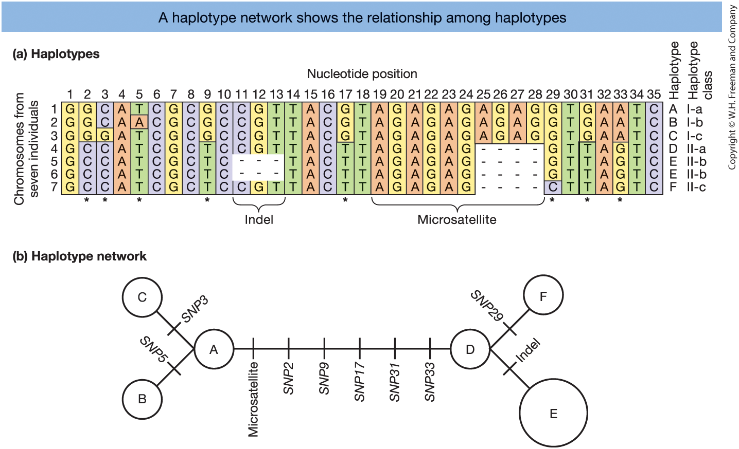
Figure 18-4.
(a) Six haplotypes (A–F) from aligned DNA sequences.
(b) Haplotype network showing mutational relationships.

• Circles = haplotypes
• Branches = mutations

Panel (a) shows aligned DNA sequences from several chromosomes. From these sequences, we identify six distinct haplotypes, labeled A through F.

Each haplotype represents a unique combination of alleles across the loci shown.

Panel (b) translates this sequence information into a haplotype network.

In the network: - Each circle represents one haplotype. - Lines connecting circles represent mutational steps. - The number of differences between haplotypes corresponds to the mutations along the branches.

Closely connected haplotypes differ by only one or a few mutations. More distant haplotypes differ at multiple sites.

This type of network helps us visualize evolutionary relationships among haplotypes.

Instead of just listing differences at individual SNPs, the network shows how haplotypes are related and how they may have evolved from one another.

Haplotype Network for Human mtDNA

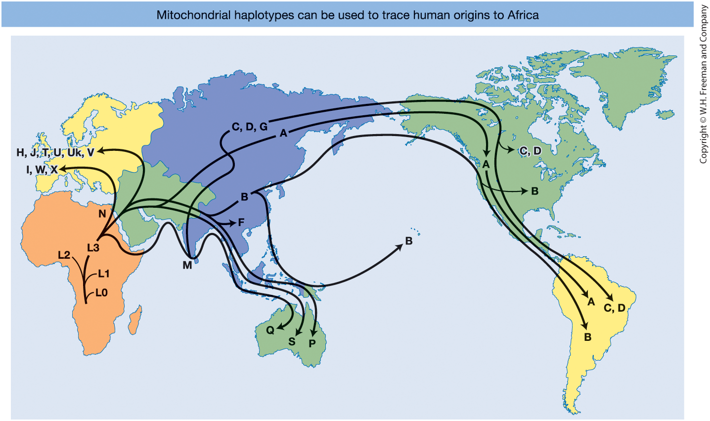
Figure 18-6 Human mitochondrial DNA haplotype network mapped globally.

• The ancestral L haplogroup appears in Africa
  
• Derived haplogroups spread worldwide
  
• Supports the Out of Africa model

This figure shows a haplotype network of human mitochondrial DNA, projected onto a world map.

Each circle represents a haplogroup. The size of a circle typically reflects its frequency. Lines connecting circles represent mutational steps.

The ancestral haplogroup, labeled uppercase L, is found in Africa. This indicates that modern human mitochondrial diversity originated in Africa.

From haplogroup L, derived lineages emerged. One important branch, L3, gave rise to haplogroups that migrated out of Africa.

These derived haplogroups spread into Europe, Asia, Oceania, and eventually the Americas.

This pattern supports the Out of Africa model of modern human origins.

The key takeaway is that haplotype networks allow reconstruction of evolutionary history and migration patterns.

Because mitochondrial DNA is inherited maternally and does not undergo recombination, it preserves clear lineage relationships over time.

2. Gene Pool Concept and Hardy–Weinberg

The Gene Pool Concept

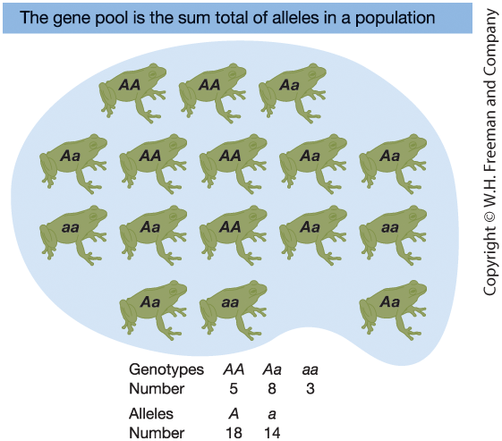
Figure 18-7. A Frog Gene Pool

Gene pool = total collection of alleles
in a population at a given time.

• Population size: N = 16 (diploid)

• Total alleles at one locus: 2N = 32

Genotype counts:

• 5 AA
  
• 8 Aa
  
• 3 aa

Allele counts:
- 18 A
- 14 a

The gene pool is the total collection of alleles in a population at a given time.

In this example, the population contains 16 frogs. Because frogs are diploid, each individual carries two alleles at this locus.

So the total number of alleles in the population is 2N, which equals 32.

The figure shows genotype counts: 5 individuals with genotype uppercase A–uppercase A, 8 with uppercase A–lowercase a, and 3 with lowercase a–lowercase a.

To describe the gene pool, we count alleles rather than genotypes.

Uppercase A–uppercase A individuals contribute two uppercase A alleles, uppercase A–lowercase a individuals contribute one uppercase A and one lowercase a, and lowercase a–lowercase a individuals contribute two lowercase a alleles.

Adding these contributions gives 18 uppercase A alleles and 14 lowercase a alleles.

This simple counting step is the basis for calculating allele frequencies.

Genotype Frequencies

Definition

Genotype frequency = proportion of individuals
with a given genotype.

For a diploid locus with alleles A and a:

\[ f(AA) = \frac{\#AA}{N} \]

\[ f(Aa) = \frac{\#Aa}{N} \]

\[ f(aa) = \frac{\#aa}{N} \]

Genotype frequencies sum to 1:

\[ f(AA) + f(Aa) + f(aa) = 1 \]

Example (N = 16 frogs)

Counts:

• 5 AA
  
• 8 Aa
  
• 3 aa

Frequencies:

\[ f(AA) = \frac{5}{16} = 0.31 \]

\[ f(Aa) = \frac{8}{16} = 0.50 \]

\[ f(aa) = \frac{3}{16} = 0.19 \]

Check: \[ 0.31 + 0.50 + 0.19 = 1 \]

Genotype frequency is the proportion of individuals with a particular genotype in the population.

It is calculated by dividing the number of individuals with that genotype by the total population size, N.

For a locus with alleles uppercase A and lowercase a, the possible genotypes are uppercase A–uppercase A, uppercase A–lowercase a, and lowercase a–lowercase a.

In the frog example, N equals 16.

So the genotype frequencies are 5 divided by 16 for uppercase A–uppercase A, 8 divided by 16 for uppercase A–lowercase a, and 3 divided by 16 for lowercase a–lowercase a.

These frequencies sum to one, because every individual must have one of these genotypes.

Genotype frequencies therefore describe how common each genotype is in the population.

Allele Frequencies

Definition

Instead of counting genotypes, we count alleles.

For a diploid population:

\[ \text{Total alleles} = 2N \]

Let:

• \(p\) = frequency of allele A
  
• \(q\) = frequency of allele a

Then:

\[ p = \frac{\#A}{2N} \qquad q = \frac{\#a}{2N} \]

Allele frequencies sum to 1:

\[ p + q = 1 \]

Example (N = 16 frogs)

Total alleles:

\[ 2N = 2 \times 16 = 32 \]

Allele counts:

• 18 A
  
• 14 a

Frequencies:

\[ p = \frac{18}{32} = 0.56 \]

\[ q = \frac{14}{32} = 0.44 \]

Check: \[ 0.56 + 0.44 = 1 \]

Instead of counting genotypes, population genetics usually counts alleles.

Because the population is diploid, each individual carries two alleles at a locus. So in a population of size N, the total number of alleles is 2N.

In this example, N equals 16 frogs, so there are 32 alleles in total.

From the genotype counts, there are 18 copies of uppercase A and 14 copies of lowercase a.

The allele frequencies are therefore p equals 18 divided by 32, and q equals 14 divided by 32.

These are the frequencies of uppercase A and lowercase a in the population.

Allele frequencies always sum to one.

The key idea is that the entire gene pool at this locus can be summarized by just two numbers: p and q.

These allele frequencies will be the starting point for the Hardy–Weinberg model.

From Alleles to Genotypes: Hardy–Weinberg Law

Hardy–Weinberg Law

If mating is random:

\[ f(AA) = p^2 \]

\[ f(Aa) = 2pq \]

\[ f(aa) = q^2 \]

\[ p^2 + 2pq + q^2 = 1 \]

If Hardy–Weinberg assumptions hold, allele frequencies remain constant across generations and the population is in equilibrium.

Why does this work?

Allele frequency = probability of drawing that allele from the gene pool.

Let:

• \(p\) = frequency of allele A
  
• \(q\) = frequency of allele a

Under random union of gametes:

\[ f(AA) = p \times p = p^2 \]

\[ f(aa) = q \times q = q^2 \]

\[ f(Aa) = p q + q p = 2pq \]

Hardy–Weinberg shows how allele frequencies determine genotype frequencies under random mating.

If the frequency of uppercase A is p, and the frequency of lowercase a is q, then genotype frequencies are

p squared for uppercase A–uppercase A, 2pq for uppercase A–lowercase a, and q squared for lowercase a–lowercase a.

These frequencies sum to one.

Why does this work?

Allele frequencies can be interpreted as probabilities. For example, p is the probability that a randomly chosen gamete carries uppercase A.

Under random union of gametes, we multiply probabilities.

The probability of uppercase A–uppercase A is p times p, which equals p squared.

The probability of lowercase a–lowercase a is q times q, which equals q squared.

For the heterozygote, there are two possible combinations: uppercase A from one parent and lowercase a from the other, or the reverse. Each occurs with probability pq, so together they give 2pq.

If the Hardy–Weinberg assumptions hold, allele frequencies remain constant across generations, and the population is in equilibrium.

If genotype frequencies deviate from these expectations, it suggests that evolutionary forces are acting.

Why Hardy–Weinberg Matters

• Provides a null model for evolution
  
• Predicts genotype frequencies from allele frequencies
  
• Allows detection of evolutionary forces
  
• Defines when a population is in equilibrium

Hardy–Weinberg is foundational in population genetics.

It provides a baseline expectation — a null model.

If observed genotype frequencies match p squared, 2pq, and q squared, the population is consistent with random mating and the absence of evolutionary forces.

If they deviate, something is acting — selection, non-random mating, drift, or structure.

Hardy–Weinberg does not explain how evolution occurs. It tells us what happens when evolutionary forces are absent.

For that reason, it is the starting point of population genetic theory.

Hardy–Weinberg: Assumptions and Violations

Hardy–Weinberg applies only if:

1. Random mating
   
2. No selection
   
3. No mutation
   
4. No migration
   
5. Infinitely large population

These conditions define the null model.

Violations occur when:

• Non-random mating
  
• Natural selection
  
• Population structure
  
• Mutation or migration
  
• Finite population size (genetic drift)

Deviations from Hardy–Weinberg
indicate evolutionary forces are acting.

Hardy–Weinberg equilibrium is a null model. It describes genotype frequencies when evolutionary forces are absent.

For the model to hold, several assumptions must be satisfied.

Mating must be random.

There must be no natural selection.

There must be no mutation and no migration.

And the population must be infinitely large. In practice, this means that random sampling effects are negligible.

If any of these assumptions are violated, genotype frequencies may deviate from Hardy–Weinberg expectations.

Non-random mating alters genotype proportions.

Selection changes genotype frequencies through differences in reproductive success.

Population structure can also create deviations. This is known as the Wahlund effect.

A finite population size introduces genetic drift, which causes random fluctuations in allele frequencies.

When deviations from Hardy–Weinberg are observed, the conclusion is that one or more evolutionary forces are acting.

From Genotype to Allele Frequencies

Mathematical relationship

At a locus with alleles A and a:

Let genotype frequencies be:

\[ f(AA), \quad f(Aa), \quad f(aa) \]

Then allele frequencies are:

\[ p = f(AA) + \tfrac{1}{2} f(Aa) \]

\[ q = f(aa) + \tfrac{1}{2} f(Aa) \]

\[ p + q = 1 \]

Intuition

Each individual carries two alleles.

• AA contributes two A alleles
  
• Aa contributes one A and one a
  
• aa contributes two a alleles

Heterozygotes contribute half to each allele.

Allele frequencies are weighted averages
of genotype frequencies.

This slide shows the reverse relationship: how to calculate allele frequencies from genotype frequencies.

Each individual carries two alleles at a locus.

Individuals with genotype uppercase A–uppercase A contribute two uppercase A alleles.

Individuals with genotype lowercase a–lowercase a contribute two lowercase a alleles.

Heterozygotes, uppercase A–lowercase a, contribute one uppercase A allele and one lowercase a allele.

Because frequencies are proportions, a heterozygote contributes half of its frequency to uppercase A and half to lowercase a.

This leads to the formulas on the slide:

p equals the frequency of uppercase A–uppercase A plus one half of the frequency of uppercase A–lowercase a,

and

q equals the frequency of lowercase a–lowercase a plus one half of the frequency of uppercase A–lowercase a.

In other words, allele frequencies are weighted averages of genotype frequencies.

These relationships allow us to move between genotype frequencies and allele frequencies, which is essential when testing Hardy–Weinberg equilibrium.

Hardy–Weinberg Test: Theory and Example

Hardy–Weinberg Test (Theory Template)

	A/A	A/G	G/G	Sum
Observed number (\(O\))	\(N_{AA}\)	\(N_{AG}\)	\(N_{GG}\)	\(N\)
Observed frequency	\(\dfrac{N_{AA}}{N}\)	\(\dfrac{N_{AG}}{N}\)	\(\dfrac{N_{GG}}{N}\)	\(1\)
Expected frequency	\(p^2\)	\(2pq\)	\(q^2\)	\(1\)
Expected number (\(E\))	\(Np^2\)	\(N(2pq)\)	\(Nq^2\)	\(N\)
\(\chi^2\) contribution	\(\dfrac{(N_{AA}-E_{AA})^2}{E_{AA}}\)	\(\dfrac{(N_{AG}-E_{AG})^2}{E_{AG}}\)	\(\dfrac{(N_{GG}-E_{GG})^2}{E_{GG}}\)	\(\chi^2\)

Estimated frequency of allele A

\[ p = \frac{2n_{AA} + n_{AG}}{2N} \]

The frequency of allele G:

\[ q = 1 - p \]

since \(p + q = 1\).

Example: SNP rs9272426 (HLA-DQA1)

	A/A	A/G	G/G	Sum
Observed number	17	55	12	84
Observed frequency	0.202	0.655	0.143	1
Expected frequency	0.281	0.498	0.221	1
Expected number	23.574	41.851	18.574	84
\(\chi^2\) contribution	1.833	4.131	2.327	8.29

Allele frequency:

\[ p = \frac{2n_{AA}+n_{AG}}{2N} = \frac{2\cdot17 + 55}{2\cdot84} = 0.53, \quad q = 0.47 \] HWE Test:

\[ \chi^2 = 8.29, \quad df = 1, \quad p = 0.004 \] Since \(p < 0.05\), the SNP deviates from Hardy–Weinberg equilibrium.

This slide shows how Hardy–Weinberg equilibrium can be tested statistically.

The general idea is simple.

First, we start with the observed genotype counts in the sample.

From these counts, we estimate the allele frequencies p and q.

Using Hardy–Weinberg expectations, we then calculate the expected genotype frequencies: p squared, 2pq, and q squared.

Multiplying these frequencies by the sample size N gives the expected genotype counts.

Next, we compare the observed and expected counts using a chi-square statistic.

For each genotype class, we calculate observed minus expected, squared, divided by expected.

Summing these contributions gives the total chi-square value.

In the example shown here, the chi-square statistic equals 8.29.

Because the allele frequency is estimated from the data, the test has one degree of freedom.

Comparing this value to the chi-square distribution gives a p-value of 0.004.

Since this is less than 0.05, the SNP deviates from Hardy–Weinberg equilibrium.

In practice, this suggests that one or more evolutionary forces may be affecting this locus.

The Chi-Square Test for Hardy–Weinberg Equilibrium

Computation

We test whether observed genotype counts deviate from Hardy–Weinberg expectations.

For each genotype class:

\[ \chi^2_i = \frac{(O - E)^2}{E} \]

• \(O\) = observed count
  
• \(E\) = expected count under HWE

Total test statistic:

\[ \chi^2 = \sum \frac{(O - E)^2}{E} \]

Inference

Compare \(\chi^2\) to the chi-square distribution with 1 degree of freedom for a biallelic locus.

If \(\chi^2\) exceeds the critical value → reject HWE.

Significant deviation suggests:

• Non-random mating
  
• Selection
  
• Population structure
  
• Genetic drift

This slide summarizes the chi-square test used to evaluate Hardy–Weinberg equilibrium.

The idea is to compare the observed genotype counts with the counts expected under Hardy–Weinberg.

For each genotype class, we calculate a chi-square contribution: the difference between observed and expected, squared, divided by the expected value.

These contributions are summed to obtain the total chi-square statistic.

For a biallelic locus, the test has one degree of freedom.

There are three genotype classes, but genotype frequencies must sum to one, and the allele frequency is estimated from the sample, which removes another degree of freedom.

The resulting chi-square value is compared to the chi-square distribution.

If the statistic is large enough, we reject Hardy–Weinberg equilibrium.

A significant deviation suggests that evolutionary forces such as selection, non-random mating, population structure, or genetic drift may be acting on the population.

3. Mating Systems and Inbreeding

Random Mating and Hardy–Weinberg

Random mating (HWE assumption)

• Individuals mate independently of genotype
  
• No genotype-based mate preference

If random mating holds:

• Genotype frequencies follow \(p^2, 2pq, q^2\)
  
• Allele frequencies remain constant

If mating is not random

Hardy–Weinberg proportions may fail.

Common causes:

• Assortative mating
  
• Disassortative mating
  
• Population subdivision
  
• Inbreeding

Non-random mating primarily alters
genotype frequencies.

Random mating is one of the central assumptions of Hardy–Weinberg equilibrium.

It means that individuals mate independently of their genotype at the locus under consideration.

Importantly, randomness is locus-specific.

Individuals may choose mates based on many traits, but as long as genotype at this particular locus does not influence mating, the assumption holds.

If random mating holds, genotype frequencies in the next generation follow p squared, 2 p q, and q squared.

Under the full Hardy–Weinberg assumptions, allele frequencies remain constant across generations.

If mating is not random, Hardy–Weinberg genotype proportions may fail.

A key insight is that non-random mating primarily changes genotype frequencies, not allele frequencies.

For example, assortative mating increases homozygosity, while disassortative mating increases heterozygosity.

Population subdivision can also produce a deficit of heterozygotes. This is known as the Wahlund effect.

Inbreeding, examined next, systematically increases homozygosity in predictable ways.

Mate Choice and Genotype Frequencies

Positive assortative mating

• Similar individuals mate
  
• Example: tall × tall

Effect:

• Excess of homozygotes
  
• Deviation from HWE proportions
  
• Allele frequencies unchanged (in the absence of other forces)

Negative assortative mating

• Dissimilar individuals mate
  
• Example: self-incompatibility (S locus) in Brassica

Effect:

• Excess of heterozygotes
  
• Deviation from HWE proportions
  
• Allele frequencies unchanged (in the absence of other forces)

Now consider how mate choice affects genotype frequencies.

In positive assortative mating, individuals preferentially mate with similar partners.

If similarity has a genetic basis, this increases the probability that identical alleles are paired in offspring.

The result is an excess of homozygotes relative to Hardy–Weinberg expectations.

Importantly, assortative mating by itself does not change allele frequencies in a single generation. It changes how alleles are combined into genotypes.

In negative assortative mating, individuals preferentially mate with genetically dissimilar partners.

This increases the probability that different alleles are paired, producing an excess of heterozygotes.

A classic example is self-incompatibility at the S locus in plants such as Brassica, where pollen carrying a matching S allele is rejected. This mechanism promotes heterozygosity.

The central point is that non-random mating alters genotype frequencies even when allele frequencies remain constant.

This distinction is essential for interpreting deviations from Hardy–Weinberg equilibrium.

Disassortative Mating: The MHC Example

Major Histocompatibility Complex (MHC)

• Central to immune recognition
  
• Highly polymorphic
  
• May influence mate choice

Evolutionary consequence

• Preference for different MHC genotypes
  
• Increased heterozygosity
  
• Potential fitness advantage

Example: HLA-DQA1 (Tuscany sample) shows heterozygote excess

	A/A	A/G	G/G	Sum
Observed number	17	55	12	84
Observed frequency	0.202	0.655	0.143	1
Expected frequency	0.281	0.498	0.221	1
Expected number	23.574	41.851	18.574	84
\(\chi^2\) contribution	1.833	4.131	2.327	8.29

This slide shows a biological example of disassortative mating.

The Major Histocompatibility Complex, or MHC, contains genes involved in immune recognition and is one of the most polymorphic regions of the genome.

In several species, including humans, MHC genotype may influence mate choice. Individuals may prefer partners with different MHC alleles.

This type of mating is called disassortative mating, because genetically dissimilar individuals are more likely to mate.

Now look at the table on the right.

The observed data show more heterozygotes than expected under Hardy–Weinberg equilibrium.

This excess of heterozygotes is consistent with disassortative mating or balancing selection favoring heterozygotes.

The key idea is that biological mechanisms such as mate choice can produce predictable deviations from Hardy–Weinberg equilibrium.

Spatial Mating and Population Structure

Isolation by distance

• Individuals mate locally
  
• Gene flow declines with distance
  
• Gradual geographic differences in allele frequencies

Population structure

• Subpopulations differ in allele frequencies
  
• Each may follow HWE locally

If pooled:

→ Excess of homozygotes
→ Wahlund effect

This slide introduces the idea of population structure.

In many species, individuals tend to mate locally. As geographic distance increases, gene flow decreases.

Over time, this creates gradual geographic differences in allele frequencies. This pattern is called isolation by distance.

More generally, a species may consist of several partially isolated subpopulations.

Each subpopulation may follow Hardy–Weinberg equilibrium locally, but with different allele frequencies.

If individuals from these subpopulations are pooled into a single sample, we often observe an excess of homozygotes.

This pattern is called the Wahlund effect.

Importantly, this deviation does not require selection or inbreeding within the subpopulations.

It can arise simply because the population actually contains hidden structure.

Therefore, when we observe a deficit of heterozygotes, one possible explanation is that the sampled individuals come from different subpopulations.

Geographic Gradients in Allele Frequency

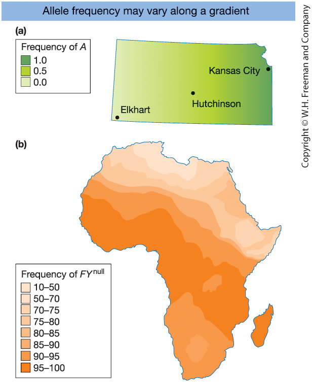
Figure 18-11

1. Hypothetical sunflower allele frequency gradient (Kansas)
   
2. Duffy blood group allele (\(FY^{0}\)) across Africa

\(\Rightarrow\) Geographic variation creates
population structure

Local HWE ≠ global HWE

These maps show geographic gradients in allele frequency, also called clines.

In panel (a), a hypothetical sunflower population shows a gradual change in allele frequency across Kansas. The frequency of the uppercase A allele varies smoothly from one region to another.

Panel (b) shows a real example: the Duffy blood group allele, pronounced F Y zero, across Africa.

This allele reaches very high frequency in parts of central Africa, where it is associated with resistance to malaria.

These patterns arise because individuals tend to mate locally, so allele frequencies can differ across geographic regions.

Each local region may follow Hardy–Weinberg equilibrium internally.

However, when individuals from different regions are pooled, the combined sample may deviate from Hardy–Weinberg expectations.

This again illustrates the effect of population structure.

The key idea is that local Hardy–Weinberg equilibrium does not necessarily imply equilibrium at the larger geographic scale.

Inbreeding

Definition

Inbreeding = mating between relatives.

Because relatives share alleles from common ancestors, offspring are more likely to inherit two identical copies of an allele.

Genetic consequences:

• Increased homozygosity
• Decreased heterozygosity
• Higher probability of expressing recessive deleterious alleles

Key concept:
Inbreeding increases homozygosity.

Biological consequences

• Increased risk of inherited disorders
  
• Possible inbreeding depression
  (reduced survival or fertility)

However, in some species inbreeding can be advantageous:

• Common in self-pollinating plants
  (e.g., rice, wheat, Arabidopsis)
  
• Preserves beneficial allele combinations
  
• Enables colonization from a single individual

The effects depend on ecological context.

Inbreeding refers to mating between related individuals.

Relatives share alleles inherited from common ancestors. As a result, their offspring have a higher probability of inheriting two copies of the same ancestral allele.

Such alleles are described as identical by descent.

The main population-genetic consequence is increased homozygosity across the genome and reduced heterozygosity.

Importantly, inbreeding changes genotype frequencies, but by itself does not change allele frequencies.

The key genetic risk is that recessive deleterious alleles are more likely to be expressed in homozygous form.

This can increase the probability of inherited disorders.

The reduction in survival or reproductive success associated with increased homozygosity is called inbreeding depression.

However, inbreeding is not always harmful.

Many plant species reproduce primarily by self-fertilization. Examples include rice, wheat, and Arabidopsis.

Self-fertilization can allow reproduction when mates are scarce, facilitate colonization, and preserve favorable allele combinations.

Overall, whether inbreeding is harmful or advantageous depends on the species, the genetic load, and the ecological context.

The central population-genetic effect remains: inbreeding increases homozygosity.

Inbreeding and Identity by Descent (IBD)

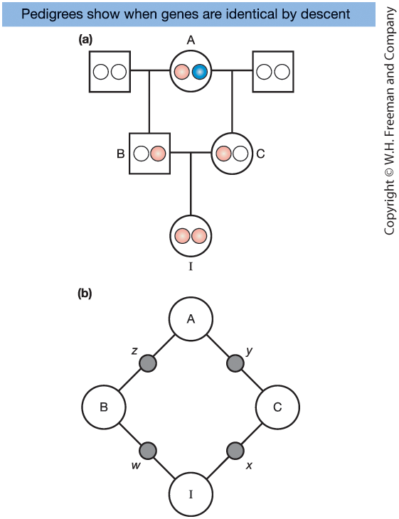
Consider the half-sib pedigree in Figure 18-12:

• B and C are half-siblings
  
• They share a common mother, A
  
• Their daughter is I

A has two gene copies:

• One from her mother (pink)
  
• One from her father (blue)

I is inbred because there is a closed ancestral loop.

• If I’s two alleles trace back to the same physical gene copy in A, they are identical by descent (IBD).

• The probability of this event is the inbreeding coefficient, \(F_I\).

Consider the pedigree shown in the Figure.

Individuals B and C are half-siblings. They share the same mother, A, but have different fathers. Their offspring is individual I.

Notice that there is a closed ancestral loop. Individual I descends from B and C, and both trace back to the same ancestor, A.

Whenever such a loop exists, the offspring may be inbred.

Now focus on individual A. She carries two physical copies of the gene, shown here as a pink copy and a blue copy.

If individual I inherits two alleles that both trace back to the same gene copy in A — either both from the pink copy or both from the blue copy — then those alleles are identical by descent.

Identical by descent means that the two alleles originate from the same ancestral gene copy.

The probability that I’s two alleles are identical by descent is called the inbreeding coefficient, denoted F sub I.

In other words, the inbreeding coefficient measures the probability of identity by descent at a locus.

Inbreeding and Genetic Disorder Risk

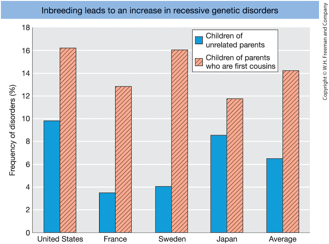
Figure 18-13 Frequency of genetic disorders among children of unrelated parents (blue columns) compared to that of children of parents who are first cousins (red columns with diagonal lines). [Data from C. Stern, Principles of Human Genetics, W. H. Freeman, 1973.]

This figure compares the frequency of genetic disorders among children of unrelated parents and children of first-cousin marriages.

Across multiple countries, the frequency of genetic disorders is consistently higher among offspring of first cousins.

In many populations, the risk is approximately doubled, although the exact increase varies across studies.

Why does this occur?

First cousins share, on average, one-eighth of their genome identical by descent.

Their children therefore have an inbreeding coefficient of F equals one over sixteen.

Because relatives share alleles inherited from common ancestors, their offspring have a higher probability of being homozygous for recessive deleterious alleles.

This increased homozygosity explains the elevated risk of inherited disorders.

Importantly, inbreeding does not create new deleterious alleles.

It increases the probability that existing recessive alleles are inherited in homozygous form and therefore expressed.

Inbreeding Increases in Small Populations

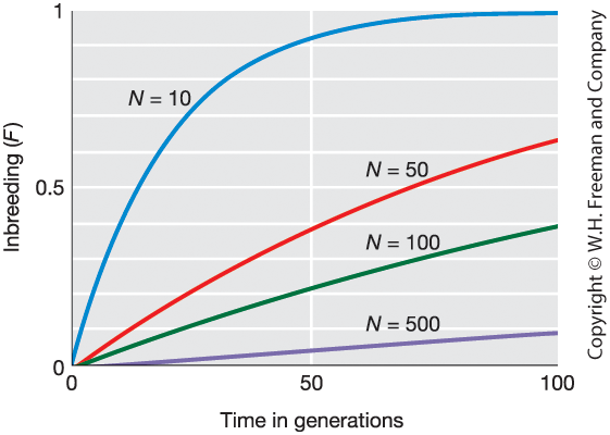
Figure 18-13

Increase in inbreeding coefficient (\(F\)) over generations for different population sizes (\(N\)).

Smaller \(N\) \(\Rightarrow\) Faster increase in \(F\)

This figure shows how the inbreeding coefficient, F, increases over time in populations of different sizes.

The key pattern is clear:

The smaller the population size, the faster inbreeding accumulates.

In very small populations, such as N equals 10, and in the absence of mutation and migration, F rises rapidly and eventually approaches one.

When F approaches one, individuals become completely homozygous because alleles have become identical by descent through drift.

In larger populations, such as N equals 500, F increases much more slowly.

This occurs because random genetic drift causes lineages to coalesce more quickly in small populations than in large ones.

Importantly, this increase in inbreeding occurs even without intentional mating between relatives.

Finite population size alone leads to increasing homozygosity over time.

This explains why small or isolated populations are at higher risk of inbreeding depression and progressive loss of genetic variation.

Genotype Frequencies Under Inbreeding

Let:

• \(p\) = frequency of allele A
  
• \(q\) = frequency of allele a
  
• \(F\) = inbreeding coefficient

Under inbreeding, genotype frequencies are:

\[ f(AA) = p^2 + Fpq \]

\[ f(Aa) = 2pq(1 - F) \]

\[ f(aa) = q^2 + Fpq \]

Interpretation

• Homozygotes increase by \(Fpq\)
  
• Heterozygotes decrease by \(2Fpq\)

If \(F = 0\) → Hardy–Weinberg

If \(F = 1\) → Complete homozygosity

Allele frequencies remain:

\[ p + q = 1 \]

The inbreeding coefficient F describes the probability that the two alleles at a locus are identical by descent.

Under Hardy–Weinberg equilibrium, genotype frequencies are p squared, 2 p q, and q squared.

Inbreeding does not change allele frequencies. Instead, it changes how alleles are paired into genotypes.

As inbreeding increases, homozygotes become more common and heterozygotes become less common.

The equations on this slide describe that change.

Each homozygote frequency increases by F p q, while the heterozygote frequency decreases by 2 F p q.

Importantly, allele frequencies remain unchanged, so p plus q still equals one.

If F equals zero, the population follows Hardy–Weinberg proportions.

If F equals one, all individuals are completely homozygous.

These equations therefore show how inbreeding alters genotype frequencies without changing allele frequencies.

Summary: Violations of Random Mating

Mechanism	Changes Allele Frequencies?	Changes Genotype Frequencies?	Typical Pattern
Positive assortative mating	No	Yes	Excess homozygotes
Negative assortative mating	No	Yes	Excess heterozygotes
Inbreeding	No (initially)	Yes	Excess homozygotes
Isolation by distance	Yes (across space)	Yes	Gradual geographic structure
Population subdivision	Yes (between groups)	Yes	Wahlund effect

This table summarizes several ways in which random mating can be violated.

The key question is whether a mechanism changes allele frequencies, genotype frequencies, or both.

Positive assortative mating and inbreeding increase homozygosity.

Negative assortative mating increases heterozygosity.

Importantly, these processes mainly change genotype frequencies, while allele frequencies may remain unchanged.

In contrast, spatial processes such as isolation by distance or population subdivision can also change allele frequencies across populations.

When individuals from genetically different groups are combined in a single sample, a deficit of heterozygotes may appear.

This pattern is known as the Wahlund effect.

The key takeaway is that deviations from Hardy–Weinberg equilibrium can arise from several different mechanisms.

Therefore, interpreting such deviations requires understanding the biological and spatial structure of the population.

4.Measurement of Genetic Variation

Measuring Genetic Variation

How do we quantify DNA variation?

For a DNA region:

1. Segregating sites (\(S\))
   Number of polymorphic nucleotide positions

2. Number of haplotypes (\(H\))
   Distinct sequence types observed

3. Allele frequencies (\(p_i\))

4. Gene diversity (expected heterozygosity)
   \[ GD = 1 - \sum p_i^2 \]
   Probability that two alleles differ

5. Nucleotide diversity (\(\pi\))
   Average pairwise nucleotide differences per site

Example: G6PD (5102 bp)

Measure	Total	Africans	Non-Africans
Sample size	47	16	31
Segregating sites	18	14	7
Haplotypes	12	9	6
Gene diversity	0.22	0.47	0.00
Nucleotide diversity (\(\pi\))	0.0006	0.0008	0.0002

Africans show higher genetic diversity.

This slide introduces common measures used to quantify DNA sequence variation.

Segregating sites, S, count the number of nucleotide positions that are polymorphic in the sample.

The number of haplotypes, H, counts the distinct DNA sequence types observed.

Allele frequencies provide the foundation for more informative measures.

Gene diversity, also called expected heterozygosity, equals one minus the sum of squared allele frequencies.

It can be interpreted as the probability that two randomly chosen alleles from the population are different.

Nucleotide diversity, pronounced pi, measures the average number of nucleotide differences between two sequences, per site.

Unlike gene diversity, which focuses on allele frequencies at a locus, pi captures sequence-level divergence across the region.

Now consider the G6PD example.

Across 5102 base pairs, only 18 sites are polymorphic. Most positions are identical across individuals.

Genetic diversity is higher in Africans than in non-Africans, both in terms of gene diversity and nucleotide diversity.

Two important lessons emerge.

First, genetic variation is sparse relative to genome length.

Second, levels of diversity can differ substantially between populations.

These statistics allow quantitative comparison of genetic variation across populations and genomic regions.

Nucleotide Diversity Across Species

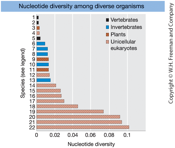
Figure 18-15

Levels of nucleotide diversity
at synonymous (silent) sites
in diverse organisms.

Key pattern:

• Vertebrates \(\Rightarrow\) low diversity
  
• Invertebrates & plants \(\Rightarrow\) moderate
  
• Many unicellular eukaryotes \(\Rightarrow\) high

This figure compares nucleotide diversity across a wide range of species.

The horizontal axis shows nucleotide diversity, pronounced pi.

Pi measures the probability that two randomly chosen DNA sequences differ at a given nucleotide site.

Several broad patterns appear.

Vertebrates, including humans and mice, generally show low nucleotide diversity.

Invertebrates and many plant species tend to show moderate levels of diversity.

Many unicellular eukaryotes show much higher diversity.

One major factor behind this pattern is effective population size.

In simple terms, nucleotide diversity increases as effective population size increases.

Species with large long-term population sizes retain more genetic variation over time.

In contrast, species with smaller populations tend to have lower genetic diversity.

The key idea is that genetic diversity reflects the long-term effective population size of a species.

5. Evolutionary Forces

Forces That Shape Genetic Variation

Fundamental evolutionary forces

• Mutation
  Generates new alleles

• Migration (gene flow)
  Moves alleles between populations

• Recombination
  Reshuffles alleles into new haplotypes

• Genetic drift
  Random sampling in finite populations

• Selection
  Differential reproductive success

What these forces determine

• Introduction of new variation
  
• Loss or fixation of alleles
  
• Changes in allele frequencies
  
• Patterns of linkage and haplotypes
  
• Genetic divergence among populations

Together, these forces determine
the evolutionary trajectory of populations.

Population genetics seeks to explain how and why allele frequencies change over time.

Five fundamental evolutionary forces govern this process.

Mutation introduces new alleles into populations. It is the ultimate source of genetic variation.

Migration, also called gene flow, moves alleles between populations and can reduce genetic differences between them.

Recombination reshuffles alleles along chromosomes, creating new haplotypes. Importantly, recombination changes combinations of alleles, but does not by itself change allele frequencies.

Genetic drift produces random fluctuations in allele frequencies because populations are finite. Its effects are strongest in small populations.

Selection changes allele frequencies systematically when some genotypes leave more offspring than others.

Together, these forces determine how genetic variation arises, how it is redistributed, how allele frequencies change, and how populations diverge through time.

They define the evolutionary dynamics of genetic variation.

Mutation: Source and Measurement

Mutation: the origin of new alleles

Mutation introduces new genetic variation into the gene pool.

• Mutation rate = probability of change per site per generation
  
• Symbol: \(\mu\)

Typical rates:

• SNPs (humans): \(\mu \approx 1\times 10^{-8}\) per site per generation
  
• Microsatellites (STRs): \(\mu \approx 10^{-4}\)–\(10^{-3}\) per locus per generation

Genome scale:

• Humans: ~50–100 new point mutations per individual per generation

Estimating mutation rates

Pedigree-based sequencing:

• Sequence parents and offspring
  
• Identify de novo mutations
  
• Count new mutations per generation

Because mutations are rare, large numbers of nucleotides must be sequenced to estimate \(\mu\) accurately.

Mutation is the ultimate source of new genetic variation. Without mutation, no new alleles would enter the gene pool.

A mutation is simply a change in the DNA sequence. We quantify mutation using the mutation rate, denoted by the symbol mu.

The mutation rate is the probability that a DNA site changes in one generation.

In humans, the mutation rate for single nucleotide polymorphisms, or SNPs, is about one times ten to the minus eight per site per generation.

Although this probability is very small, the human genome contains about three billion base pairs. As a result, each individual carries roughly fifty to one hundred new point mutations in every generation.

Other genetic markers mutate much faster. Microsatellites, also called short tandem repeats, have mutation rates around ten to the minus four to ten to the minus three per locus per generation.

How do we estimate mutation rates?

One common approach is pedigree sequencing. We sequence the genomes of parents and their offspring, and identify mutations that appear in the child but not in either parent. These are called de novo mutations.

Because mutations are rare, large amounts of DNA must be sequenced to estimate mutation rates accurately.

Mutation is therefore rare at each site, but across the whole genome it continuously introduces new genetic variation.

Migration (Gene Flow) and Admixture

Migration (gene flow)

Movement of individuals or gametes
between populations that reproduce successfully.

Consequences:

• Introduces new alleles into populations
  
• Changes allele frequencies
  
• Increases within-population variation
  
• Reduces genetic divergence among populations
  
• Counteracts genetic drift

Genetic admixture

Gene flow between previously separated populations.

• Individuals inherit ancestry from multiple populations
  
• Genomes become mosaics of ancestry segments
  
• Common in humans and many species

Admixture is the genomic signature of migration.

In addition to mutation, migration is a fundamental evolutionary force.

Migration, also called gene flow, occurs when individuals or gametes move between populations and contribute offspring to the recipient population.

When migrants reproduce successfully, they introduce new alleles into the population.

This directly changes allele frequencies.

Gene flow typically increases genetic variation within populations and reduces genetic differences among populations.

In this sense, migration counteracts genetic drift, which tends to cause populations to diverge over time.

The genomic consequence of migration is admixture.

When previously separated populations interbreed, their descendants inherit DNA from multiple ancestral sources.

As a result, individual genomes become mosaics, containing chromosomal segments derived from different populations.

These ancestry segments can be identified using genome-wide genetic markers.

Admixture therefore provides a measurable genomic signature of historical migration events.

Migration and Genetic Admixture

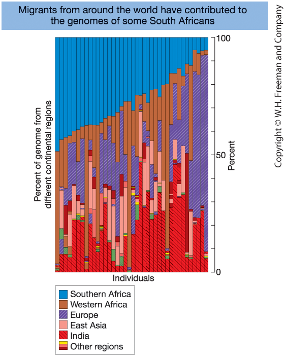
Figure 18-16. Genetic admixture in individuals of mixed ancestry (South Africa).

Each vertical bar represents one individual.
Colors indicate genomic segments inherited
from different ancestral populations.

Admixture reflects historical migration
and interbreeding between populations.

This figure illustrates genetic admixture, which is the genomic signature of migration.

Each vertical bar represents one individual.

The different colors show the proportion of that individual’s genome inherited from different ancestral populations.

Importantly, individuals do not belong to a single ancestry category.

Instead, their genomes are mosaics, composed of chromosomal segments derived from multiple ancestral sources.

This pattern arises when previously separated populations interbreed over generations.

Migration introduces alleles from different populations.

Recombination then reshuffles the genome each generation, breaking chromosomes into smaller ancestry segments.

Over time, these ancestry tracts become shorter, but the mixed ancestry signal remains detectable.

This figure illustrates a key principle:

Migration increases genetic variation within populations and reduces sharp genetic boundaries between populations.

Admixture therefore provides direct genomic evidence of historical gene flow.

Recombination and New Haplotypes

Parental haplotypes (before recombination)

Consider two linked loci:

• Locus A: A / a
  
• Locus B: B / b

Suppose the original haplotypes are:

• \(AB\)
  
• \(ab\)

Because the loci are physically close, these allele combinations are often inherited together.

Recombinant haplotypes (after crossover)

A crossover between loci A and B can generate:

• \(Ab\)
  
• \(aB\)

Recombination:

• Does not create new alleles
  
• Creates new combinations of existing alleles
  
• Reduces linkage disequilibrium
  
• Increases haplotype diversity

Over time, recombination reshapes associations between loci.

Recombination reshuffles alleles between loci during meiosis.

Importantly, recombination does not create new alleles. Only mutation introduces new alleles into the gene pool.

Instead, recombination creates new combinations of alleles that already exist.

In this example, the original haplotypes are uppercase A–uppercase B and lowercase a–lowercase b.

Because the two loci are physically close, these allele combinations are often inherited together.

If a crossover occurs between the loci, two new haplotypes can be produced: uppercase A–lowercase b and lowercase a–uppercase B.

These are called recombinant haplotypes.

Recombination therefore increases haplotype diversity without changing allele frequencies.

Over time, recombination also reduces linkage disequilibrium, the statistical association between alleles at different loci.

In this way, recombination continually reshapes the genetic structure of populations.

Linkage Disequilibrium (LD)

Linkage equilibrium

Two loci are in linkage equilibrium
when alleles combine independently.

If independent:

\[ P_{AB} = p_A p_B \]

The haplotype frequency
equals the product of allele frequencies.

Linkage disequilibrium (LD)

If:

\[ P_{AB} \neq p_A p_B \]

alleles are associated non-randomly
across loci.

Measuring LD

For two biallelic loci (A/a and B/b):

• Observed haplotype frequency: \(P_{AB}\)
• Expected under independence: \(p_A p_B\)

Define:

\[ D = P_{AB} - p_A p_B \]

Interpretation:

• \(D = 0\) → linkage equilibrium
  
• \(D > 0\) → excess of \(AB\) haplotypes
  
• \(D < 0\) → deficit of \(AB\) haplotypes

\(D\) measures the magnitude and direction
of statistical association between loci.

Linkage equilibrium means that alleles at two loci combine independently when forming haplotypes.

If the frequency of allele uppercase A is p sub A, and the frequency of allele uppercase B is p sub B, then the expected frequency of haplotype uppercase A–uppercase B is p sub A multiplied by p sub B.

This follows the basic multiplication rule of probability.

Linkage disequilibrium occurs when this independence is violated.

If the observed frequency of the haplotype uppercase A–uppercase B differs from p sub A times p sub B, the alleles are statistically associated.

The statistic D measures this deviation.

D equals the observed haplotype frequency minus the expected frequency under independence.

If D equals zero, the loci are in linkage equilibrium.

If D is positive, the uppercase A–uppercase B haplotype occurs more often than expected.

If D is negative, it occurs less often than expected.

Linkage disequilibrium can arise from several processes, including physical linkage, selection, genetic drift, or population structure.

Dynamics of Linkage Disequilibrium

How LD arises

LD arises when alleles become associated
non-randomly across loci.

Common causes:

• A new mutation appears on a single chromosome
  → initially in strong LD with nearby alleles

• Migration (admixture) mixes populations
  with different haplotype frequencies

• Genetic drift in finite populations

New alleles typically begin in LD
with their chromosomal background.

LD decay by recombination

Recombination breaks down
non-random associations.

Let \(r\) = recombination fraction between loci.

\[ D_{t+1} = (1-r)D_t \]

• Small \(r\) (tight linkage) → slow decay
  
• Large \(r\) (loose linkage) → rapid decay
  
• \(r = 0.5\) → fastest decay (independent assortment)

Over generations:

\[ D_t = (1-r)^t D_0 \]

Linkage disequilibrium is dynamic. It is constantly being created and broken down.

First, how does LD arise?

When a new mutation appears, it occurs on a single chromosome. That chromosome carries specific neighboring alleles, so the mutation initially shows strong linkage disequilibrium with its surrounding genetic background.

LD can also arise through migration. If individuals from different populations mix, their haplotype structures may differ, creating non-random allele associations.

Genetic drift in small populations can also generate LD through random sampling.

Now consider how LD decays.

Recombination breaks apart haplotypes during meiosis.

The equation on the slide shows that each generation LD is reduced by a factor of one minus r, where r is the recombination fraction between the loci.

If r is small, meaning the loci are tightly linked, LD decays slowly.

If r is large, meaning recombination is frequent, LD decays more rapidly.

Over multiple generations, LD declines approximately exponentially.

In this way, LD reflects a balance between forces that create allele associations and recombination, which gradually erodes them.

Random Genetic Drift: Simulation Results

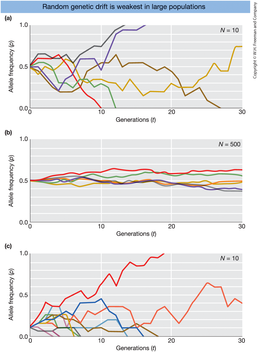
Figure 18-18
Simulations of random genetic drift

Each colored line = one simulated population
tracked for 30 generations.

1. Small population (\(N = 10\), \(p_0 = 0.5\))
   
2. Large population (\(N = 500\), \(p_0 = 0.5\))
   
3. Small population (\(N = 10\), \(p_0 = 0.1\))

Hardy–Weinberg assumes an infinitely large population.

Real populations are finite.

In finite populations, allele frequencies change by chance:

Random genetic drift

This figure shows simulations of random genetic drift.

Each colored line represents one population, tracked across generations.

All populations begin with the same allele frequency, but they evolve differently because each generation is formed by random sampling.

In panel (a), the population size is small, with N equal to 10 and an initial allele frequency of 0.5.

Allele frequencies fluctuate strongly. Some populations reach fixation, while others lose the allele entirely.

Panel (b) shows a much larger population, with N equal to 500.

Here the fluctuations are much smaller, and allele frequencies change more slowly.

Panel (c) again shows a small population, but the allele begins at a low frequency.

Most populations quickly lose the allele, because rare alleles are easily lost by chance.

The key principle is that genetic drift is strongest in small populations.

Hardy–Weinberg equilibrium assumes an infinitely large population, but real populations are finite.

Because of random sampling, allele frequencies fluctuate across generations.

These random fluctuations are called genetic drift, and they can lead to fixation or loss of alleles even without natural selection.

Natural Selection and Fitness

Natural selection

Individuals with certain heritable traits
are more likely to survive and reproduce.

Key ingredients:

• Genetic variation exists in populations
  
• Traits are heritable
  
• Individuals differ in reproductive success
  
• Alleles associated with higher reproduction increase in frequency

Evolution = change in allele frequencies over generations.

Fitness

Darwinian fitness = reproductive success.

Absolute fitness (\(W\)):
Expected number of offspring produced.

Relative fitness (\(w\)):
Fitness relative to the most successful genotype.

Example:

If the most successful genotype produces 10 offspring:

• 10 offspring → \(w = 1.0\)
  
• 5 offspring → \(w = 0.5\)

Selection acts through differences in fitness.

Natural selection explains how populations adapt over time.

Selection occurs when individuals with certain heritable traits survive or reproduce more successfully than others.

For natural selection to operate, three conditions must be met.

First, genetic variation must exist in the population.

Second, traits must be heritable.

Third, individuals must differ in reproductive success.

When these conditions are met, alleles associated with higher reproductive success increase in frequency across generations.

Fitness describes reproductive success.

Absolute fitness, denoted uppercase W, is the expected number of offspring produced.

Relative fitness, denoted lowercase w, expresses fitness relative to the most successful genotype, which is assigned a value of one.

Relative fitness determines how allele frequencies change over time.

In population genetics, evolution is defined as a change in allele frequencies across generations.

Natural selection produces those changes when genotypes differ in fitness.

Example: Selection on a Dominant Beneficial Allele

Genotype fitnesses

Genotype	Relative fitness (\(w\))
A/A	1.0
A/a	1.0
a/a	0.5

Allele A is beneficial and dominant.

Only \(a/a\) individuals have reduced fitness.

Effect on allele frequency

After selection:

• A/A and A/a survive equally well
  
• \(a/a\) individuals contribute fewer offspring

Result:

• Frequency of allele A increases
  
• Frequency of allele a decreases

Selection reduces the frequency
of the low-fitness genotype.

In this example, allele uppercase A is beneficial and dominant.

Both uppercase A–uppercase A and uppercase A–lowercase a individuals have full relative fitness equal to one.

Only lowercase a–lowercase a individuals have reduced fitness.

Because these individuals produce fewer offspring, fewer copies of allele lowercase a are passed to the next generation.

As a result, the frequency of allele uppercase A increases, while the frequency of allele lowercase a decreases.

An important principle follows.

When a beneficial allele is dominant, selection acts directly against the recessive genotype.

However, once the recessive allele becomes rare, it is mostly found in heterozygotes.

Because heterozygotes have full fitness, selection removes the recessive allele only slowly.

As a result, the recessive allele can persist at low frequency in the population.

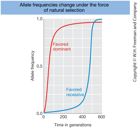
Selection and Allele Frequency

Figure 18-21

Change in allele frequency over time for:

• Favored dominant allele (red)
  
• Favored recessive allele (blue)

Both alleles increase due to natural selection, but at different rates.

This figure shows how natural selection changes allele frequencies over time.

In both cases, the allele shown is beneficial.

However, one allele is dominant and the other is recessive.

The dominant beneficial allele, shown in red, increases rapidly at the beginning.

This happens because the allele is expressed even when rare, in heterozygous individuals.

Selection can therefore act on it immediately.

In contrast, the recessive beneficial allele, shown in blue, increases very slowly at first.

When rare, it is mostly found in heterozygotes, where its beneficial effect is not expressed.

Selection can only act on the allele when it appears in homozygous form.

Once the allele becomes more common, homozygotes appear more frequently and the increase accelerates.

The key idea is that dominance influences the speed at which beneficial alleles spread.

General Model of Selection

Allele Frequency After Selection

For two alleles A and a:

Genotype fitnesses:

\[ w_{AA}, \quad w_{Aa}, \quad w_{aa} \]

Mean fitness:

\[ \bar{w} = p^2 w_{AA} + 2pq w_{Aa} + q^2 w_{aa} \]

Allele frequency in next generation:

\[ p' = \frac{p^2 w_{AA} + pq\, w_{Aa}}{\bar{w}} \]

Interpretation

• Selection acts on genotypes, not alleles
  
• Genotypes with higher fitness contribute more offspring
  
• The numerator counts transmission of allele A after selection
  
• The denominator rescales by mean population fitness

If \(w_{AA}\) and \(w_{Aa}\) are high → allele A increases

If \(w_{aa}\) is low → allele a decreases

Selection changes allele frequencies
through differences in reproductive success.

This equation describes the general model for allele frequency change under natural selection.

We begin with genotype frequencies p squared, two p q, and q squared.

Each genotype has a relative fitness: w sub A A, w sub A a, and w sub a a.

After selection, genotypes with higher fitness contribute more offspring to the next generation.

The average reproductive success of the population is called the mean fitness, denoted w-bar.

To obtain the allele frequency in the next generation, we count how often allele uppercase A is transmitted after selection.

Allele uppercase A is passed on by uppercase A–uppercase A individuals and by uppercase A–lowercase a individuals.

This gives the numerator in the equation for p prime.

The denominator, w-bar, rescales the population so that genotype frequencies sum to one.

The key principle is that selection acts on genotypes, but allele frequencies change because genotypes differ in fitness.

If one genotype consistently has higher fitness, its associated allele will increase in frequency across generations.

Example: Selection on a Dominant Beneficial Allele

Genotype	HW freq	Fitness (\(w\))	After selection	Normalized freq (\(f'\))
A/A	0.01	1.0	0.01	0.017
A/a	0.18	1.0	0.18	0.303
a/a	0.81	0.5	0.405	0.681

Assume initial allele frequencies:

\[ p = 0.10, \qquad q = 0.90 \]

Under Hardy–Weinberg:

\[ p^2 = 0.01,\quad 2pq = 0.18,\quad q^2 = 0.81 \]

Mean fitness:

\[ \bar{w} = 0.01 + 0.18 + 0.405 = 0.595 \]

New Allele Frequency

\[ p' = f'(AA) + \tfrac12 f'(Aa) \]

\[ p' = 0.017 + 0.152 = 0.169 \]

\[ 0.10 \rightarrow 0.17 \]

Interpretation

• Selection reduces contribution of \(a/a\)
• A-containing genotypes transmit more alleles
• Allele A increases in frequency

Selection changes allele frequencies
through differential reproductive success.

This table shows step by step how natural selection changes allele frequencies.

First, we calculate genotype frequencies under Hardy–Weinberg equilibrium.

With p equal to 0.10 and q equal to 0.90, the genotype frequencies are

p squared equals 0.01, two p q equals 0.18, and q squared equals 0.81.

Next, each genotype frequency is multiplied by its relative fitness.

This gives genotype frequencies after selection, but before normalization.

The sum of these values is the mean fitness of the population, denoted w-bar.

Because the genotype a–a has lower fitness, the total is reduced.

To obtain proper frequencies, we divide each value by the mean fitness. This normalization step ensures that genotype frequencies sum to one.

Finally, we calculate the new allele frequency.

Allele uppercase A is contributed by A–A individuals and by half of the A–a individuals.

This gives p prime equal to approximately 0.17.

So in one generation, the allele frequency increases from 0.10 to about 0.17.

The key idea is that selection acts on genotypes, but allele frequencies change because genotypes differ in reproductive success.

Forms of Selection

Natural selection

Directional selection

• Allele frequency moves toward fixation or loss
  
• Positive selection: favors beneficial alleles
  
• Purifying selection: removes deleterious alleles

Balancing selection

• Maintains multiple alleles in the population
  
• Example: heterozygote advantage
  
• Produces stable equilibrium allele frequencies

Artificial selection

Selection imposed by humans.

• Individuals with desired traits are chosen
  
• Those individuals contribute more offspring
  
• Favored alleles increase in frequency

Examples:

• Dog breeds
  
• Dairy cattle
  
• Crop varieties

Artificial selection = natural selection
directed by humans.

Natural selection can operate in several different ways.

Directional selection changes allele frequencies in a consistent direction.

Positive selection increases the frequency of beneficial alleles, sometimes leading to fixation.

Purifying selection, also called negative selection, removes deleterious alleles from the population.

Both of these are forms of directional selection.

Balancing selection operates differently.

Instead of eliminating one allele, it maintains multiple alleles within the population.

A classic example is heterozygote advantage, where heterozygotes have higher fitness than either homozygote.

In this case, selection maintains a stable equilibrium of allele frequencies.

Selection can also be imposed by humans.

In artificial selection, individuals with desirable traits are chosen to reproduce.

Over generations, alleles associated with those traits increase in frequency.

Dogs, dairy cattle, and many crop varieties are products of artificial selection.

The genetic mechanism is the same as natural selection. The difference is that humans decide which traits are favored.

Selective Sweep and Genetic Variation

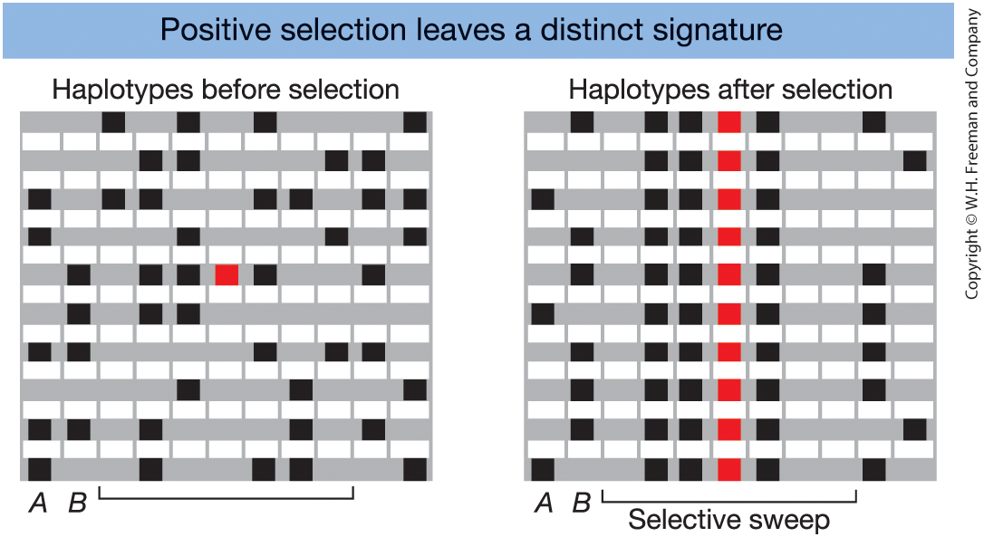
Figure 18-22

Haplotypes before and after
a beneficial allele (red)
sweeps to fixation.

After selection:

• Reduced genetic diversity
  
• Increased linkage disequilibrium
  
• One dominant haplotype

This figure illustrates a selective sweep.

Before selection, many different haplotypes exist in the population, and genetic diversity is high in the region.

A new beneficial mutation appears, shown in red.

Because the mutation increases fitness, natural selection drives it rapidly toward fixation.

The mutation originates on a single chromosome, so nearby alleles on that chromosome are carried along with it.

This process is called genetic hitchhiking.

As the beneficial allele spreads, the surrounding chromosomal segment also becomes common in the population.

As a result, genetic diversity near the selected site decreases, and one dominant haplotype becomes common.

At the same time, linkage disequilibrium increases, because nearby alleles are strongly associated.

Farther from the selected site, recombination breaks these associations, and genetic diversity gradually returns.

The key idea is that positive selection can reduce genetic variation locally, creating a characteristic genomic signature of low diversity and high linkage disequilibrium.

Selective Sweep and Genetic Variation

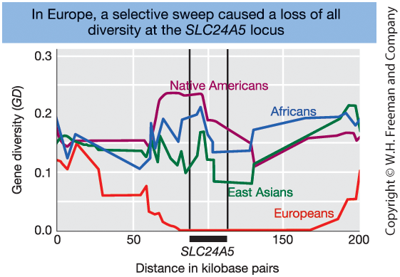
Figure 18-23. Gene diversity near the SLC24A5 locus on chromosome 15.

Gene diversity is strongly reduced in Europeans
around the SLC24A5 locus.

This pattern is consistent with
a recent selective sweep.

This figure shows a real genomic example of a selective sweep.

The horizontal axis shows genomic position along a region of chromosome 15.

The vertical axis shows gene diversity, which measures the probability that two randomly chosen alleles differ.

The gene SLC24A5 is located near the center of this region. This gene is involved in skin pigmentation.

In European populations, gene diversity drops sharply around this locus.

In contrast, African, East Asian, and Native American populations show much higher diversity in the same region.

This pattern is consistent with a recent selective sweep in European populations.

A beneficial mutation increased rapidly in frequency, and nearby alleles were carried along with it. This process is called genetic hitchhiking.

Because the sweep occurred relatively recently, recombination has not yet restored genetic variation around the selected site.

The key idea is that strong positive selection can produce a localized reduction in genetic diversity.

Examples of Natural Selection in Humans

Gene	Trait / Function	Population(s)
G6PD	Malaria resistance	African populations
HBB (β-globin)	Malaria resistance (sickle-cell trait)	African, Mediterranean, South Asian populations
CCR5	Reduced susceptibility to HIV	European populations
LCT	Lactase persistence (milk digestion)	European and some African populations
SLC24A5	Skin pigmentation	European populations
MHC	Infectious disease resistance	Multiple populations

These genes show evidence of recent natural selection.

This table shows several well-known examples of natural selection in human populations.

Many involve resistance to infectious diseases.

For example, variants in the G6PD gene and in the HBB gene, which includes the sickle-cell allele, provide protection against malaria.

In the case of sickle-cell, heterozygotes gain protection against malaria, while homozygotes can develop severe disease. This is a classic example of balancing selection.

Other examples involve adaptation to diet.

The LCT gene allows adults to digest lactose. In populations with a long history of dairy farming, alleles for adult milk digestion increased in frequency.

This illustrates gene–culture coevolution.

SLC24A5 provides an example related to skin pigmentation. Allele frequencies vary geographically, consistent with adaptation to different levels of ultraviolet radiation.

Finally, the MHC region shows very high genetic diversity across human populations, reflecting balancing selection driven by infectious disease.

The key message is that natural selection has shaped human genetic variation in the recent past, and evolutionary processes continue to operate today.

Balancing Selection Maintains Genetic Diversity

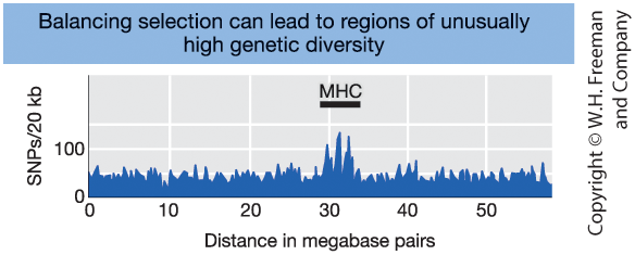
Figure 18-24

Number of SNPs along chromosome 6.

The MHC region shows a pronounced spike
of unusually high genetic diversity.

Key idea:
Balancing selection can maintain multiple alleles at a locus.

Directional selection often reduces genetic diversity.

When a beneficial allele sweeps to fixation, nearby genetic variation is lost.

Balancing selection has the opposite effect.

Instead of eliminating variation, it maintains multiple alleles in the population.

This figure shows the number of SNPs along a region of chromosome 6.

Most regions of the genome show moderate levels of diversity.

However, the MHC region shows a striking spike of unusually high genetic diversity.

The MHC, or Major Histocompatibility Complex, contains genes involved in immune recognition.

One explanation for this elevated diversity is heterozygote advantage.

Individuals carrying two different MHC alleles may recognize a wider range of pathogens.

As a result, selection favors maintaining multiple alleles rather than fixing a single variant.

The key idea is that balancing selection maintains genetic diversity at the selected locus.

This pattern is the opposite of a selective sweep.

Mutation Maintains Genetic Variation

Neutral Variation: Mutation vs Drift

• Mutation creates new alleles
  
• Genetic drift removes variation

In small populations:

• Drift is strong
  
• Diversity is low

In large populations:

• Drift is weak
  
• Diversity is higher

Key idea:
Genetic diversity reflects a balance between mutation and drift.

Deleterious Alleles: Mutation vs Selection

• Mutation continuously creates harmful alleles
  
• Natural selection removes them

Even harmful alleles persist at low frequency
because mutation never stops.

Stronger selection → lower frequency
Higher mutation rate → higher frequency

Key idea:
Mutation prevents genetic variation from disappearing completely.

Mutation is the ultimate source of new genetic variation.

But why does variation not disappear, and why does it not increase indefinitely?

First, consider neutral variation.

Mutation introduces new alleles, while genetic drift removes variation through random sampling.

In small populations, drift is strong, so genetic diversity tends to be low.

In large populations, drift is weaker, and more variation can be maintained.

Genetic diversity therefore reflects a balance between mutation adding variation and drift removing it.

Now consider deleterious alleles.

Mutation continuously produces harmful mutations, while natural selection removes them.

However, mutation never stops.

As a result, deleterious alleles persist at low frequencies in the population.

Stronger selection keeps these alleles rarer, while higher mutation rates increase their frequency slightly.

The key idea is that mutation maintains genetic variation even when other evolutionary forces remove it.

Without mutation, genetic variation would eventually disappear.

6. Applications of Population Genetics

Biological and Social Applications

Real-world applications

Population genetics informs:

• Conservation biology
  • Managing genetic diversity
    
  • Preventing inbreeding depression
    
  • Designing sustainable breeding programs
• Medical genetics
  • Estimating carrier and disease risk
    
  • Understanding recessive disorders
    
  • Interpreting GWAS findings
• Forensic science
  • Calculating DNA match probabilities
    
  • Accounting for population structure

Core principles applied

These applications rely on:

• Allele frequencies
  
• Hardy–Weinberg equilibrium
  
• Inbreeding and genetic drift
  
• Linkage disequilibrium
  
• Natural selection

Population genetics connects

DNA variation → population patterns → real-world decisions.

Population genetics is not only theoretical. Its principles are applied widely in biology and society.

In conservation biology, small populations are vulnerable to genetic drift and inbreeding. Genetic analysis helps maintain diversity, reduce inbreeding depression, and design sustainable breeding strategies.

In medical genetics, Hardy–Weinberg equilibrium is used to estimate carrier frequencies for recessive disorders. Mutation–selection balance explains why some disease alleles persist in populations. Linkage disequilibrium forms the foundation of genome-wide association studies.

In forensic science, DNA match probabilities are calculated using allele frequencies and Hardy–Weinberg assumptions. Population structure must be considered carefully to avoid biased probability estimates.

The key message is this:

Population genetics links molecular variation to population-level patterns and ultimately to practical decisions in conservation, medicine, and law.

Conservation Genetics

Genetic Risks in Small Populations

When population size declines:

• Genetic bottlenecks reduce diversity
  
• Genetic drift removes alleles randomly
  
• Inbreeding increases homozygosity
  
• Recessive deleterious alleles become expressed

Consequences:

• Reduced adaptive potential
  
• Increased risk of inbreeding depression
  (reduced survival or reproduction)

Management Dilemma

Key question:

Should conservation programs
minimize inbreeding
or allow inbreeding to purge deleterious alleles?

Theoretical argument:

• Inbreeding exposes harmful alleles
  
• Selection may remove some of them (“purging”)

Empirical evidence:

• Inbreeding often reduces fitness
  
• Maintaining genetic diversity is generally safer

Conservation genetics examines the genetic consequences of small population size.

When populations decline sharply, genetic bottlenecks reduce variation in a single generation.

Genetic drift becomes stronger, randomly eliminating alleles.

In small populations, individuals are also more likely to mate with relatives, increasing inbreeding.

Inbreeding increases homozygosity across the genome.

As homozygosity rises, recessive deleterious alleles are more likely to be expressed.

This can lead to inbreeding depression, which means reduced survival, reduced fertility, or both.

A long-standing debate concerns purging.

The theoretical idea is that inbreeding exposes harmful alleles, allowing natural selection to remove them from the population.

In principle, this could reduce genetic load over time.

However, empirical studies show that inbreeding more often reduces population fitness than successfully eliminates deleterious alleles.

For this reason, most conservation strategies aim to:

Increase effective population size, maintain gene flow between populations, and preserve genetic diversity.

The central objective is to maintain long-term evolutionary potential.

Population Genetics in Medicine

Why Allele Frequencies Matter

Population genetics allows us to:

• Estimate carrier frequencies
• Calculate disease risk
• Predict the impact of inbreeding
• Interpret population screening data

Using Hardy–Weinberg equilibrium:

• Genotype frequencies can be inferred
  from allele frequencies
• Carrier frequencies can be estimated
  without pedigrees

Example: Recessive Disease

Under Hardy–Weinberg:

• Disease frequency = \(q^2\)
• Allele frequency = \(q = \sqrt{q^2}\)
• Carrier frequency = \(2pq\)

Effect of inbreeding:

\[ \text{Homozygote frequency} = q^2 + Fpq \]

• \(F\) = inbreeding coefficient
  
• Inbreeding increases homozygosity
  
• Recessive disease risk increases

Population genetics allows us to estimate disease risk at the population level, even without detailed family pedigrees.

Consider a recessive disorder.

Under Hardy–Weinberg equilibrium, the frequency of affected individuals equals q squared.

If we observe the disease frequency, we can calculate the allele frequency q by taking the square root.

Once we know q, we can compute the carrier frequency.

Under Hardy–Weinberg, the carrier frequency equals 2 p q.

These calculations are widely used in genetic counseling and population screening programs.

Now consider inbreeding.

Inbreeding increases the probability that two alleles are identical by descent.

Under inbreeding, the homozygote frequency becomes

q squared plus F p q.

The additional term, F p q, represents the excess homozygotes caused by inbreeding.

This explains why consanguineous marriages increase the risk of recessive disorders.

The key point is:

Population genetic theory provides a quantitative framework for estimating medical risk.

DNA Forensics

Genetic Basis of Forensic Analysis

DNA identification relies on:

• Microsatellite markers (STRs)
  Highly polymorphic, multi-allelic loci

• Population allele frequencies
  Estimated from reference databases

• Hardy–Weinberg equilibrium
  Used to calculate genotype probabilities

Multiple independent loci are analyzed
to increase discriminatory power.

Statistical Interpretation

We evaluate the random match probability:

\[ P(\text{match} \mid \text{unrelated individual}) \]

This is the probability that a random person
would share the same DNA profile.

Assuming independence across loci:

• Genotype probabilities are multiplied
  
• Overall probability becomes extremely small

Very small probability → strong statistical evidence

DNA evidence does not prove guilt directly. It provides statistical evidence.

Forensic analysis typically uses short tandem repeats, or STR markers.

STRs are highly polymorphic, meaning they have many alleles. This makes them highly informative for distinguishing individuals.

To evaluate a match, we use population allele frequency databases.

Under Hardy–Weinberg equilibrium, we calculate genotype probabilities at each locus.

For heterozygotes, the probability equals 2 p q. For homozygotes, it equals p squared.

Assuming loci are independent — that is, in linkage equilibrium — we multiply probabilities across loci.

This produces the random match probability:

The probability that a random, unrelated individual would share the same DNA profile.

With many STR markers, this probability can become extremely small — often one in millions or billions.

Population genetics therefore converts a DNA match into a quantitative statistical statement.

The reliability of this statement depends on:

Accurate allele frequency estimates, appropriate population reference data, and correct assumptions about independence.

Summary Population Genetics

What We Observe

• DNA sequence variation
  
• Allele and genotype frequencies
  
• Linkage disequilibrium
  
• Population differences

Represent measurable genetic patterns.

The Null Model

Hardy–Weinberg equilibrium

• Random mating
  
• Infinite population (no drift)
  
• No mutation, migration, or selection

Deviations indicate evolutionary forces.

Evolutionary Forces

• Mutation
  
• Migration (gene flow)
  
• Recombination
  
• Genetic drift
  
• Natural selection

Change in allele frequencies over time

What These Forces Shape

• Genetic diversity
  
• Population structure
  
• Linkage disequilibrium
  
• Genomic signatures of history
  
• Medicine, conservation, and forensics

Population genetics connects patterns → processes → consequences

This slide summarizes the entire chapter within a single conceptual framework.

Start in the upper left.

Population genetics begins with observable patterns: DNA variation, allele frequencies, genotype distributions, linkage disequilibrium, and differences between populations.

These are measurable quantities.

However, patterns alone do not explain themselves.

That is where the null model comes in.

Hardy–Weinberg equilibrium defines what we expect in the absence of evolutionary forces.

If mating is random, the population is infinitely large, and no mutation, migration, or selection occurs, allele frequencies remain constant.

This defines no evolutionary change.

When real populations deviate from this expectation, we infer that evolutionary forces are operating.

Those forces are listed in the lower left panel.

Mutation introduces new alleles. Migration moves alleles between populations. Recombination reshuffles alleles. Genetic drift changes frequencies randomly in finite populations. Natural selection changes them non-randomly.

In population genetics, evolution has a precise definition: a change in allele frequencies across generations.

Finally, the lower right panel shows what these forces shape.

They determine levels of genetic diversity, the structure of populations, patterns of linkage disequilibrium, and the genomic signatures of past events.

They also inform applications in medicine, conservation biology, and forensic science.

The central idea of this chapter is:

Population genetics explains why genetic patterns look the way they do, by connecting observable variation to the evolutionary processes that shape it.

That is the framework of the field.