Center for Quantitative Genetics and Genomics
Aarhus University
2026-03-27
1. Measuring Quantitative Variation
2. A Simple Genetic Model
3. Heritability
4. Mapping Quantitative Traits
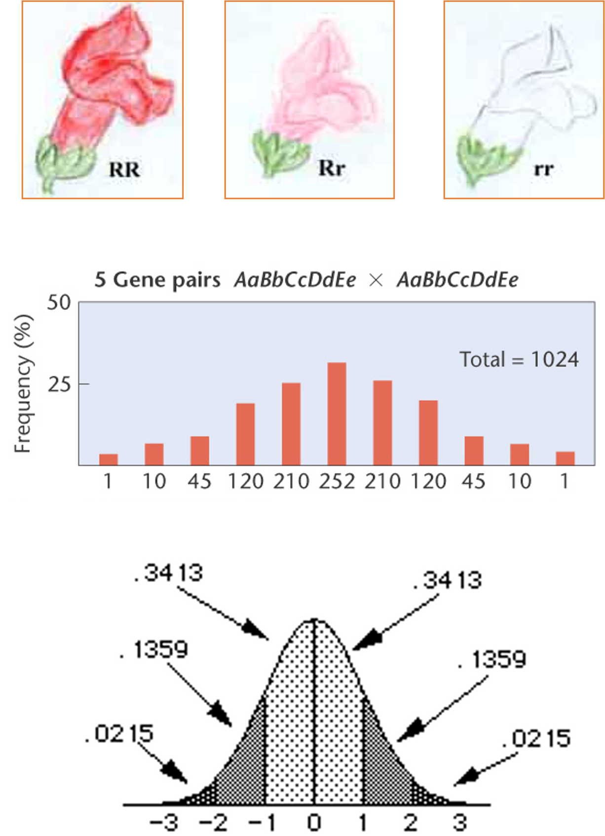
Quantitative genetics studies complex traits influenced by many genes and environmental factors.
It extends Mendelian genetics by focusing on the combined effects of many genes and the environment.
Statistical models are central to its analysis.
A biological discipline with great applied significance for agriculture, human healthcare, and for understanding evolutionary processes.
Core concepts
Relevant for genetic analyses
Natural selection and selective breeding can both cause changes in animals and plants:
Natural selection happens naturally.
Selective breeding occurs when humans intervene => artificial selection.
Selective breeding (and natural selection) takes place over many generations.
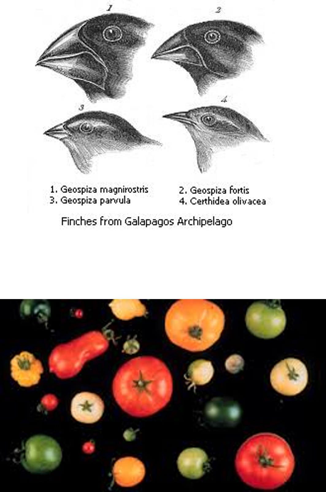
Phenotype (P) is determined by genotype (G) and environment (E):
\[ P = G + E \]
Quantitative genetics asks:
How much of the phenotypic variation is due to genetic differences?
This leads to the concept of heritability.
Why does this matter?
Quantitative genetics allows us to:
In all cases, we seek to estimate the effect of genotypes (\(G\)) on phenotypes (\(P\)).
Mendelian traits
Quantitative traits

Individuals are described by their phenotype (e.g., appearance, performance, or disease status).
Continuous traits
Categorical traits
Threshold traits
Meristic traits
To study complex traits, we need basic statistical tools:
These tools allow us to quantify and compare phenotypic variation.
Mean
\[ \bar{x} = \frac{1}{n} \sum_{i=1}^{n} x_i \]
Variance
\[ \mathrm{Var}(X) = \frac{1}{n-1} \sum_{i=1}^{n} (x_i - \bar{x})^2 \]
Normal distribution
\[ f(x) = \frac{1}{\sqrt{2\pi\sigma^2}} \exp\left(-\frac{(x-\mu)^2}{2\sigma^2}\right) \]
When studying quantitative traits, we usually sample from a population.
Sample mean:
\[ \bar{X} = \frac{1}{n} \sum_{i=1}^{n} X_i \]
Population mean:
\[ \mu \]
The mean describes the center of the data.
Example
Height (cm) for 5 individuals:
168, 172, 170, 174, 166
\[ \bar{X} = \frac{168 + 172 + 170 + 174 + 166}{5} \]
\[ \bar{X} = \frac{850}{5} = 170 \]
We use \(\bar{X}\) to estimate the true population mean \(\mu\).
Variance describes the spread of the data.
Deviation from the mean:
\[ d_i = X_i - \bar{X} \]
Population variance:
\[ \sigma^2 = \frac{\sum (X_i - \mu)^2}{n} \]
Standard deviation:
\[ \sigma = \sqrt{\sigma^2} \]
Example
Using the sample: 168, 172, 170, 174, 166
Mean: \[ \bar{X} = 170 \]
Deviations: -2, 2, 0, 4, -4
Squared deviations: 4, 4, 0, 16, 16 (sum = 40)
Variance (n = 5): \[ \sigma^2 = \frac{40}{5} = 8 \]
Standard deviation: \[ \sigma = \sqrt{8} \approx 2.83 \text{ cm} \]
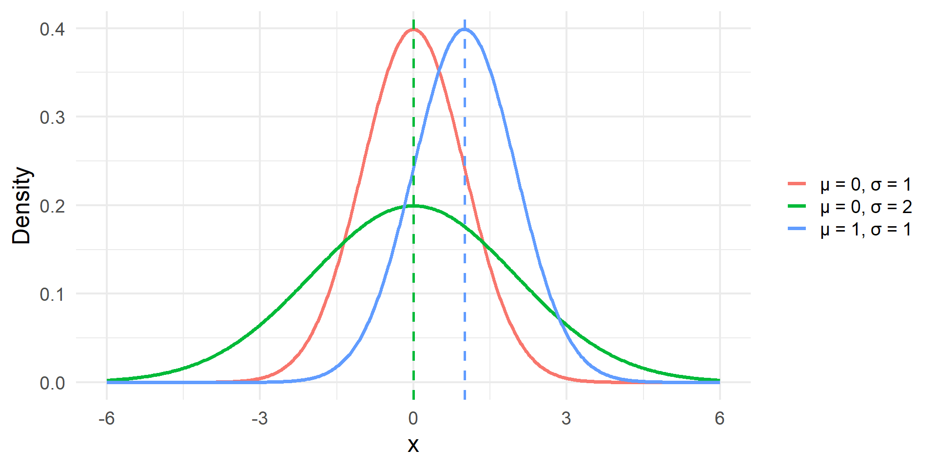
Many biological traits follow an approximately normal distribution.
A normal distribution is fully determined by:
Probability density function:
\[ f(x) = \frac{1}{\sigma \sqrt{2\pi}} \exp\left( -\frac{(x - \mu)^2}{2\sigma^2} \right) \]
Key Properties
Central role in quantitative genetics
Model
A quantitative trait can be expressed as:
\[ P = \mu + G + E \]
Deviation from the mean:
\[ p = P - \mu = G + E \]
Interpretation
Differences between individuals arise from:
This model underlies:
Step 1: Observed phenotype
Step 2: Deviation from the mean
\[ p = P - \mu \]
\[ p = 229 - 170 = 59 \text{ cm} \]
He is 59 cm taller than average.
Step 3: Interpret using the genetic model
Recall:
\[ p = G + E \]
Therefore:
\[ 59 = G + E \]
The deviation must arise from:
We observe only the total deviation — not its separate components.

Why this matters
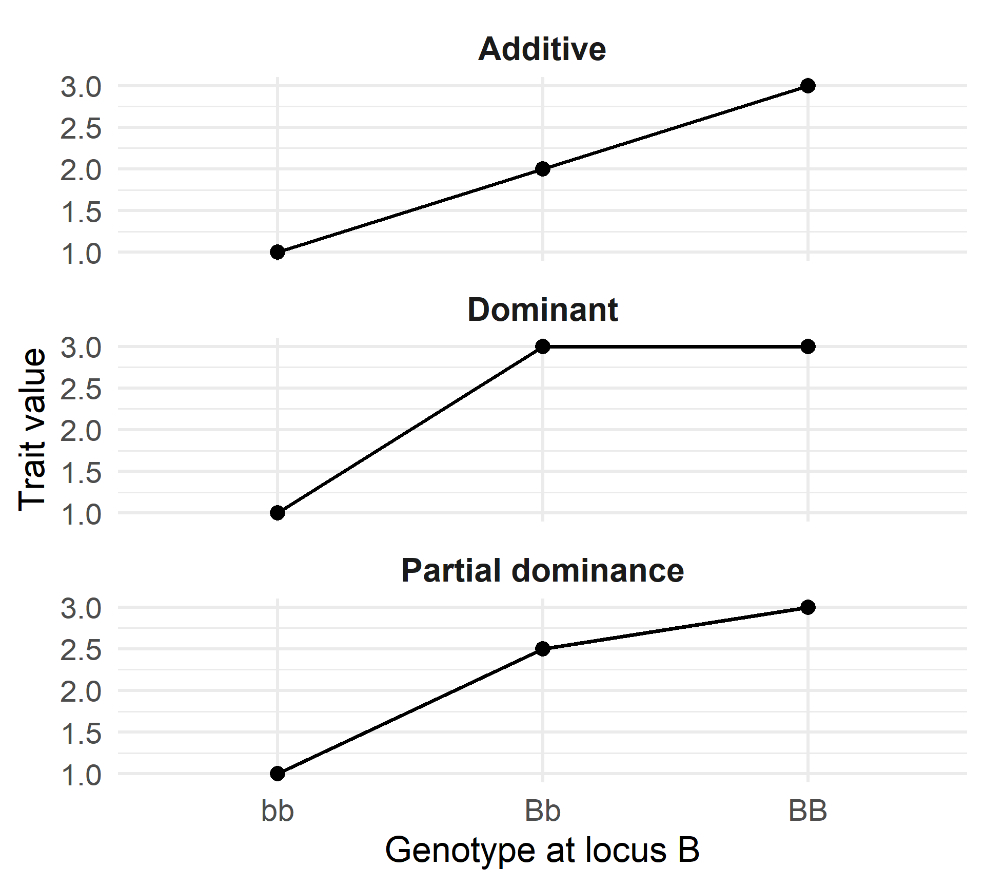
Additive gene action:
Dominance:
Key insight:
Only additive effects contribute to narrow-sense heritability

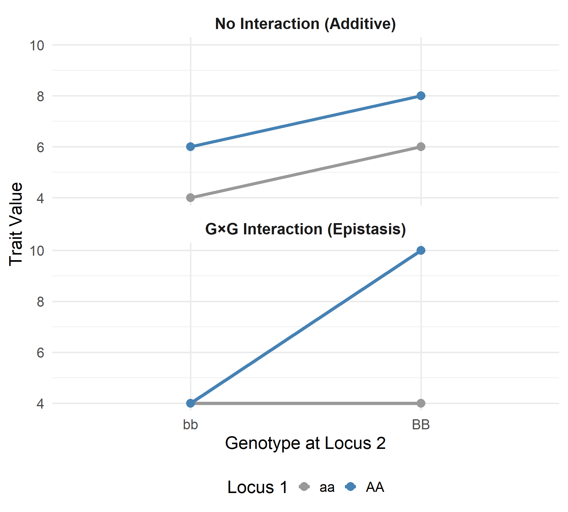
Interaction between Locus 1 and Locus 2
No Interaction (Additive)
G\(\times\)G Interaction (Epistasis)
Key Idea:
The phenotypic expression of one gene is modified by the presence of another gene.

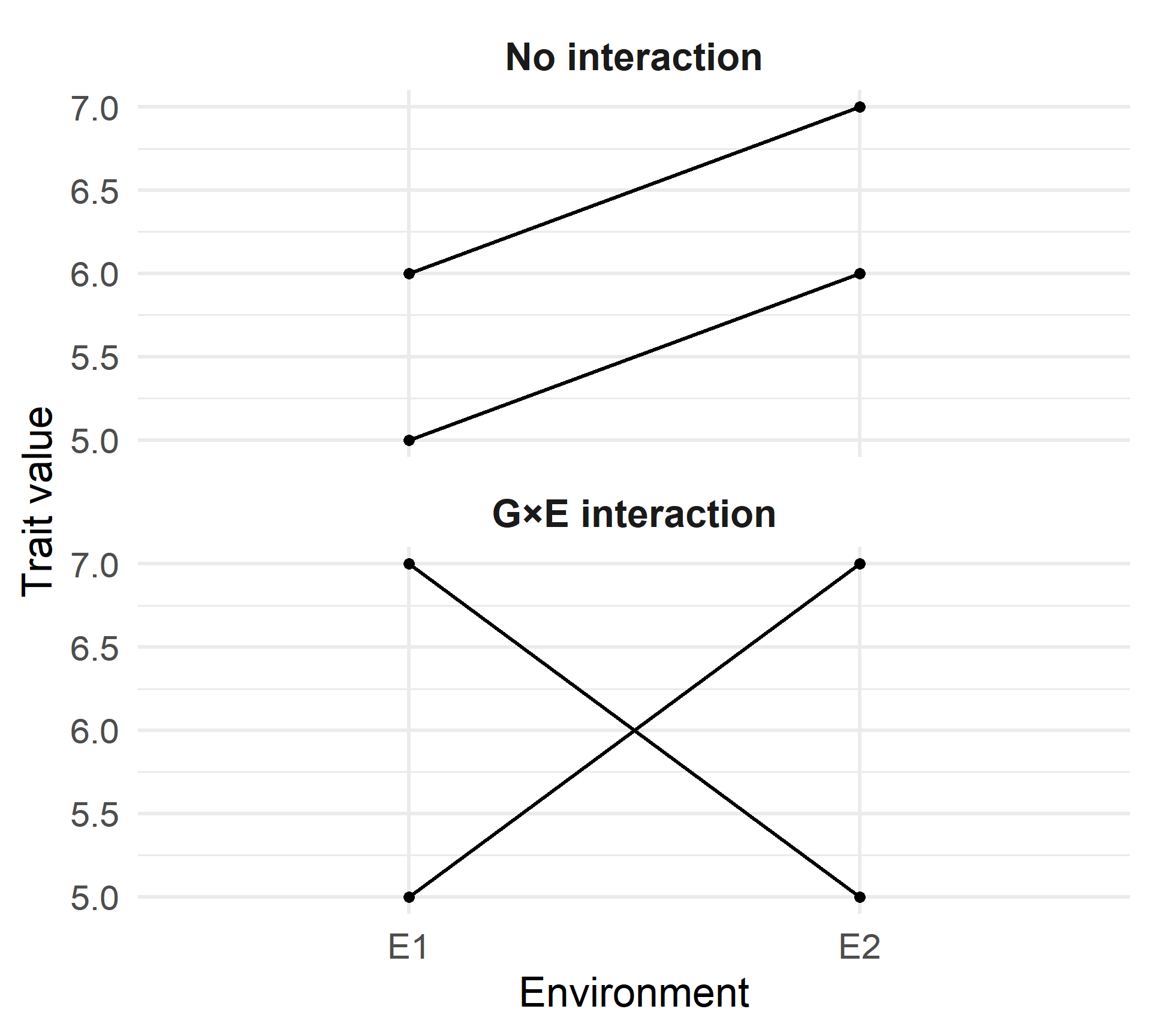
No interaction
G×E interaction
Key idea:
Genotype performance can be environment-dependent.
Start with the model
\[ P = \mu + G + E \]
Phenotypic variance:
\[ V_P = \mathrm{Var}(P) \]
Since \(\mu\) is constant:
\[ V_P = \mathrm{Var}(G + E) \]
Basic statistical rule:
\[ V_P = V_G + V_E + 2\mathrm{Cov}(G,E) \]
If genetic and environmental effects are independent
\[ \mathrm{Cov}(G,E) = 0 \]
Then:
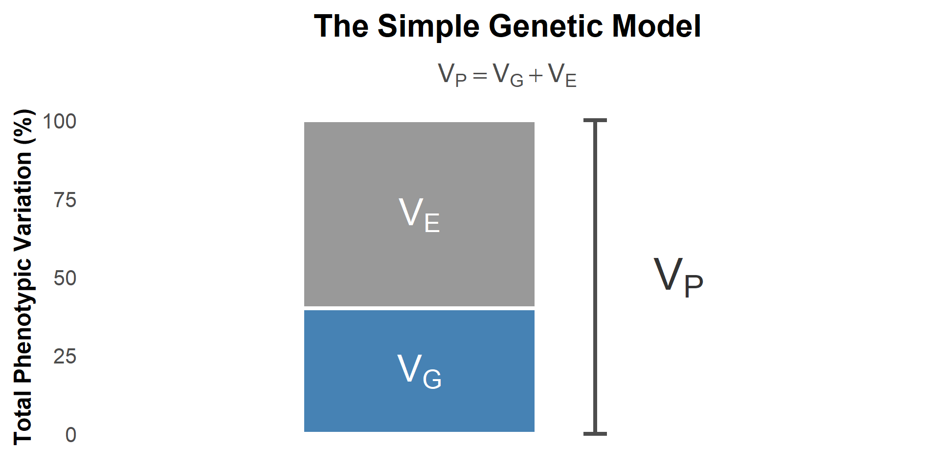
\[ V_P = V_G + V_E \]
Meaning:
Total variation = genetic variation + environmental variation
This is the foundation of heritability.
Numerical results
Total phenotypic variance:
\[ V_P = 14.67 \]
Genetic variance
(variation among inbred line means):
\[ V_G = 12.00 \]
Environmental variance
(variation among environments):
\[ V_E = 2.67 \]
Check:
\[ V_P = V_G + V_E = 12.00 + 2.67 = 14.67 \]
Interpretation
Most variation is genetic
(12.00 of 14.67)
Environmental variation is smaller
(2.67)
The decomposition holds because:
\[ \mathrm{Cov}(G,E) = 0 \]
Genotypes were randomized
across environments
This illustrates that variance components add when genotype and environment are independent.
Covariance: The Core Quantity
Covariance measures whether two variables vary together:
\[ \mathrm{Cov}(X,Y) \]
It appears everywhere in Quantitative Genetics:
Variance is simply:
\[ \mathrm{Var}(X) = \mathrm{Cov}(X,X) \]
Standardized Form: Correlation
Correlation rescales covariance:
\[ r = \frac{\mathrm{Cov}(X,Y)}{\sigma_X \sigma_Y} \]
In the variance model:
\[ V_P = V_G + V_E + 2\mathrm{Cov}(G,E) \]
If Cov(G,E) = 0, variance components add cleanly.
Definition
Key question:
Broad-sense heritability:
\[ H^2 = \frac{V_G}{V_P} \]
where:
Range:
Interpretation
Important:
“Broad-sense” includes:
Experiment I: Similar Environments
\[ H^2 = \frac{12.0}{14.67} = 0.82 \]
Interpretation:
Experiment II: More Variable Environments
\[ H^2 = \frac{12.0}{36.0} = 0.33 \]
Interpretation:
Theory
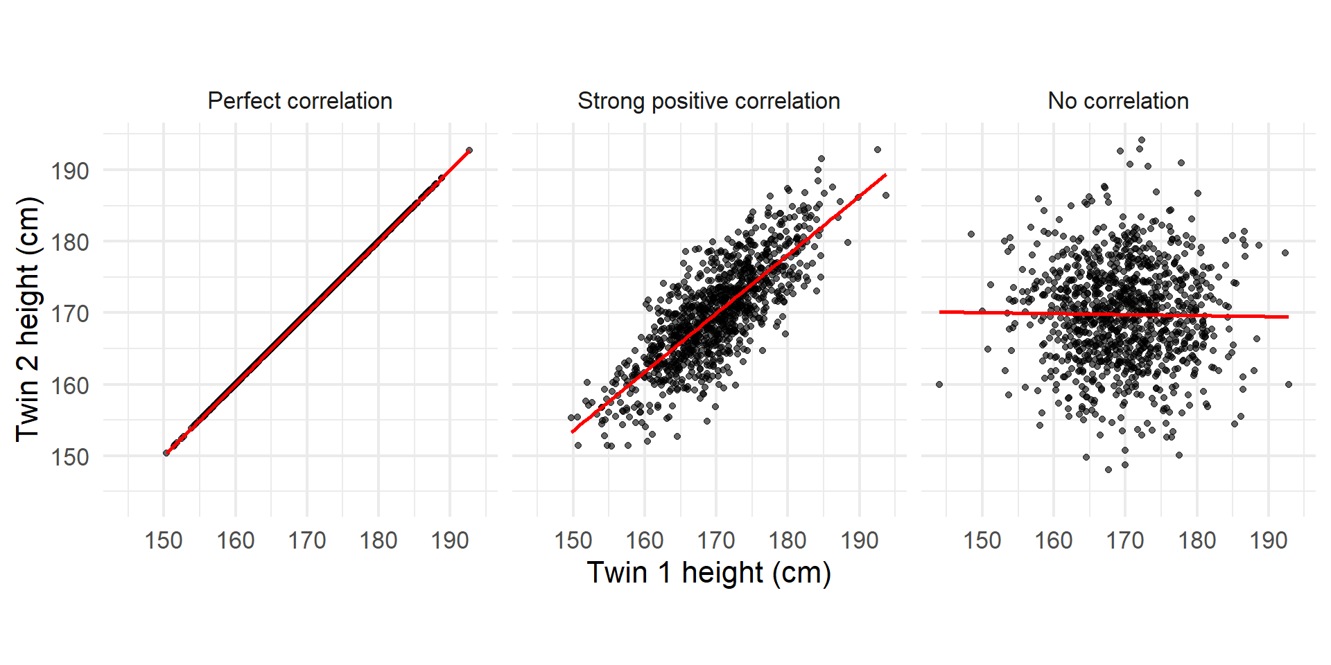
Identical (monozygotic) twins:
Under independence:
\[ \mathrm{Cov}(\text{Twin 1}, \text{Twin 2}) = V_G \]
Therefore:
\[ H^2 = \frac{V_G}{V_P} = \frac{\mathrm{Cov}(\text{twins})}{V_P} \]
Key assumption:
\[ \mathrm{Cov}(G,E) = 0 \]
Example: IQ in Twins Reared Apart
From data:
Heritability estimate:
\[ H^2 = \frac{119.2}{154.3} = 0.77 \]
Interpretation
77% of IQ variation (in this population)
is associated with genetic differences
Refers to population variation
— not individuals
| Trait | \(H^2\) |
|---|---|
| Physical traits | |
| Height | 0.88 |
| Fingerprint ridge count | 0.97 |
| Systolic blood pressure | 0.64 |
| Cognitive traits | |
| IQ | 0.69 |
| Spatial processing speed | 0.36 |
| Personality traits | |
| Extraversion | 0.54 |
| Neuroticism | 0.48 |
| Psychiatric disorders | |
| Autism | 0.90 |
| Schizophrenia | 0.80 |
| Major depression | 0.37 |
| Beliefs / attitudes | |
| Religiosity (adults) | 0.30–0.45 |
| Conservatism (adults) | 0.45–0.65 |
This table shows broad-sense heritability (\(H^2\)) estimates from twin studies.
\[ H^2 = \frac{V_G}{V_P} \]
Key patterns:
Physical traits → often high \(H^2\)
(e.g., height, fingerprints)
Cognitive & personality traits → moderate \(H^2\)
Psychiatric disorders → variable
(some high, some moderate)
Even beliefs and attitudes show measurable heritability
From Broad to Narrow Heritability
Broad-sense heritability:
\[ H^2 = \frac{V_G}{V_P} \]
But genetic variance contains multiple components:
Additive variance (\(V_A\))
→ predictably transmitted
Dominance variance (\(V_D\))
→ depends on allele combinations
Total genetic variance:
\[ V_G = V_A + V_D + V_I \]
where \(V_I\) = interaction (epistatic) variance
Narrow-Sense Heritability
\[ h^2 = \frac{V_A}{V_P} \]
Focuses only on additive variance.
Why?
Key idea:
Additive genetic variation drives response to selection.
Definition
\[ h^2 = \frac{V_A}{V_P} \]
Only additive variance is predictably transmitted.
Broad-sense heritability:
\[ H^2 = \frac{V_G}{V_P} \]
But:
\[ V_G = V_A + V_D + V_I \]
Estimation
Parent–offspring covariance:
\[ \mathrm{Cov}_{\text{parent, offspring}} = \frac{1}{2} V_A \]
Therefore:
\[ h^2 = \frac{2\,\mathrm{Cov}_{\text{parent, offspring}}}{V_P} \]
Half-sibs share \(\frac{1}{4}\) of additive effects:
\[ V_A = 4\,\mathrm{Cov}_{\text{half-sibs}} \]
Example:
Human height: \(h^2 \approx 0.8\)

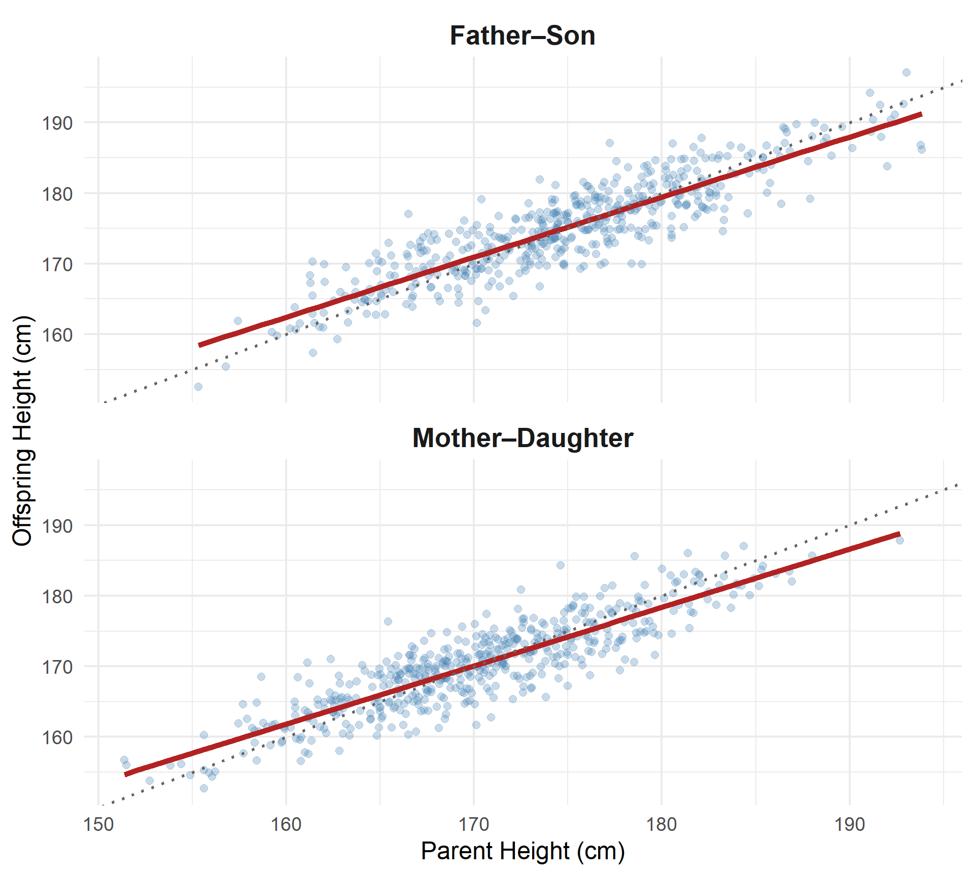
Parent–Offspring Regression for Height
Interpretation:
The steeper the slope, the greater the additive genetic contribution to variation.
| Trait | h² (%) |
|---|---|
| Agronomic species | |
| Body weight (cattle) | 65 |
| Milk yield (cattle) | 35 |
| Back-fat thickness (pig) | 70 |
| Litter size (pig) | 5 |
| Body weight (chicken) | 55 |
| Egg weight (chicken) | 50 |
| Natural species | |
| Bill length (Darwin’s finch) | 65 |
| Flight duration (milkweed bug) | 20 |
| Plant height (jewelweed) | 8 |
| Fecundity (red deer) | 46 |
| Life span (collared flycatcher) | 15 |
These are estimates of narrow-sense heritability (h²) in different species and traits.
\[h^2 = V_A / V_P\]
Patterns:
Low h² does not mean genes are unimportant —
it means additive variance is limited relative to total variance.
What is transmitted?
Individual deviation from the mean:
\[ x = a + d + e \]
Parents:
\[ x' = a' + d' + e' \]
\[ x'' = a'' + d'' + e'' \]
Expected offspring deviation:
\[ \mathbb{E}[x_0] = \frac{a' + a''}{2} \]
Only additive effects (\(a\))
are predictably transmitted.
Dominance (\(d\)) and environment (\(e\))
are not transmitted predictably.
Prediction Using \(h^2\)
Since \(a\) is not directly observed:
\[ \widehat{x}_{\text{offspring}} = h^2 \,\bar{x}_{\text{parents}} \]
Predicted phenotype:
\[ \widehat{X}_{\text{offspring}} = \mu + \widehat{x}_{\text{offspring}} \]
Example (Sheep fleece)
Population mean = 6.0 lb
Mean parental deviation = 0.75
\(h^2 = 0.4\)
\[ 0.4 \times 0.75 = 0.3 \]
Predicted offspring:
\[ 6.0 + 0.3 = 6.3 \text{ lb} \]
Artificial selection
Humans select individuals with desirable phenotypes for reproduction.
Selection differential \[ S = \bar{X}_{\text{selected}} - \bar{X}_{\text{population}} \]
Response to selection \[ R = \bar{X}_{\text{offspring}} - \bar{X}_{\text{population}} \]
Breeder’s equation \[ R = h^2 S \qquad h^2 = \frac{R}{S} \]
Only additive genetic variance contributes to the response.
Example: Provitamin A in maize
Base population mean = 1.25 µg/g
Selected mean = 1.63 µg/g
Offspring mean = 1.44 µg/g
Selection differential:
\[ S = 1.63 - 1.25 = 0.38 \]
Response:
\[ R = 1.44 - 1.25 = 0.19 \]
Heritability:
\[ h^2 = \frac{0.19}{0.38} = 0.50 \]
About 50% of the variation contributing to selection is additive and transmitted to the next generation.

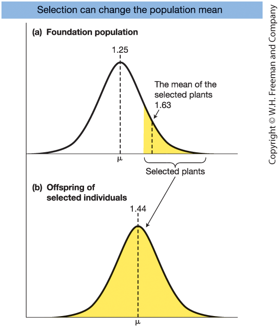
Figure 19-9.
One generation of artificial selection for provitamin A in maize.
Base population mean = 1.25 μg/g
Selected group mean = 1.63 μg/g
Offspring mean = 1.44 μg/g
Selection differential:
\[
S = 1.63 - 1.25 = 0.38
\]
Selection response:
\[
R = 1.44 - 1.25 = 0.19
\]
Only the additive (heritable) component causes the shift in the next generation.

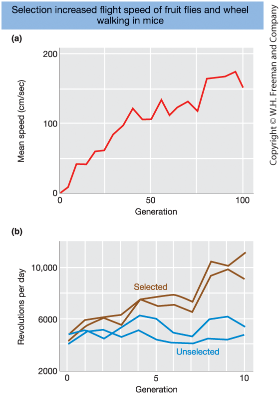
Figure 19-10.
Long-term selection experiments demonstrate sustained evolutionary change.
Key message:
Populations contain substantial additive genetic variation
and can respond to selection for many generations.
Broad-sense heritability \[ H^2 = \frac{V_G}{V_P} \]
Narrow-sense heritability \[ h^2 = \frac{V_A}{V_P} \]
Heritability is:
Heritability does NOT mean:
What we know so far
The Big Question
The Solution: Association Mapping
We move from describing how much is inherited
to identifying what is inherited.
Goal
Identify genomic regions associated with complex traits
in natural, random-mating populations.
Core Idea
Test statistical associations between:
Key Characteristics
Compared to classical QTL mapping

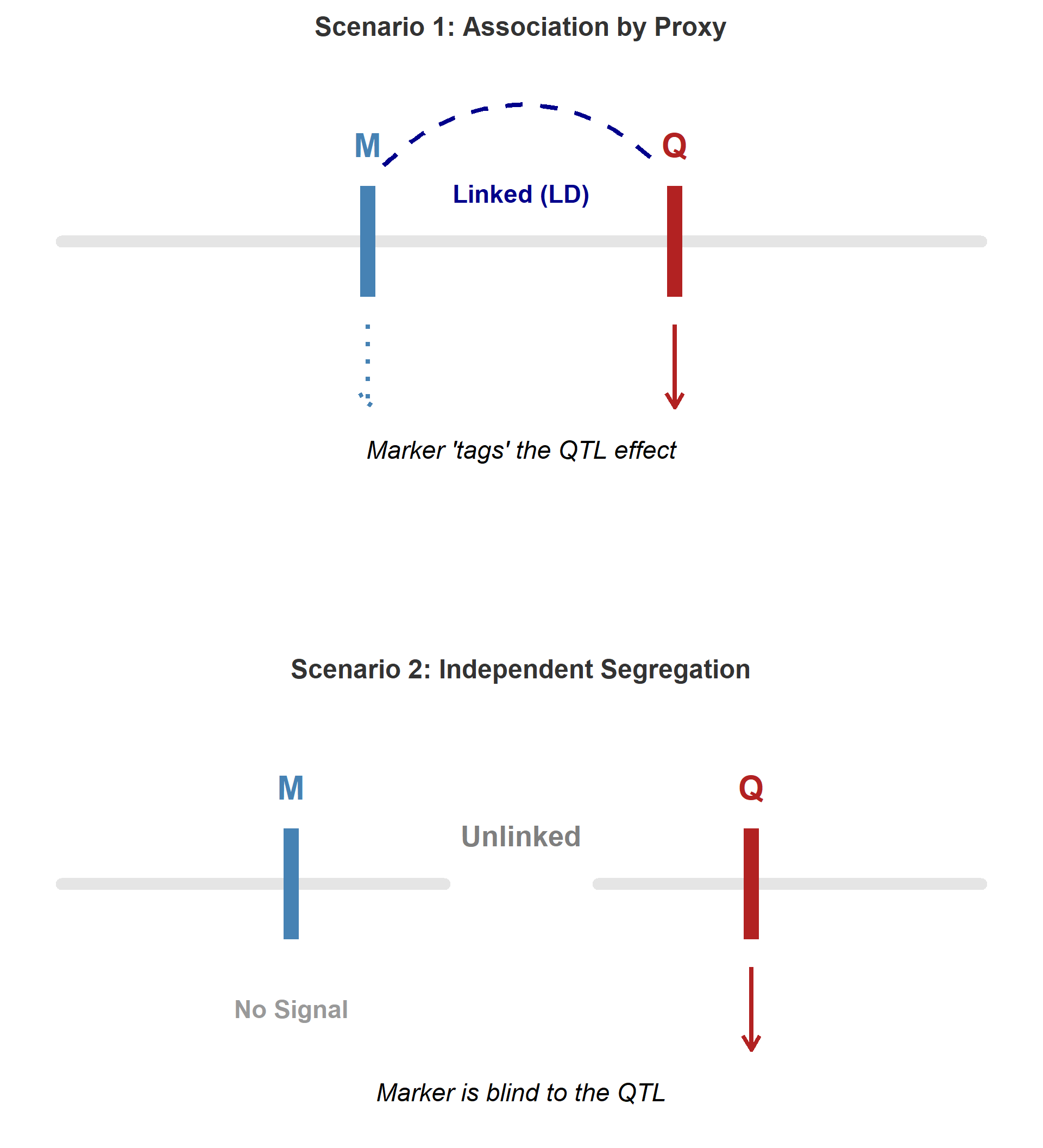
Concept
Therefore, the SNP shows statistical association
even if it is not itself causal.
Key Point
GWAS detects markers that are in LD
with causal variants.
Phenotype data
Measured trait values for \(n\) individuals.
Example (height):
| Individual | Phenotype (\(y\)) |
|---|---|
| Ind₁ | 170 |
| Ind₂ | 165 |
| Ind₃ | 182 |
| … | … |
Phenotypes form a vector:
\[ \mathbf{y} = \begin{pmatrix} y_1 \\ y_2 \\ y_3 \\ \vdots \end{pmatrix} \]
Genotype matrix
Genotypes organized into an \(n \times m\) matrix.
| SNP₁ | SNP₂ | SNP₃ | … | |
|---|---|---|---|---|
| Ind₁ | 0 | 1 | 2 | |
| Ind₂ | 1 | 1 | 0 | |
| Ind₃ | 2 | 0 | 1 | |
| … |
Common SNP coding:
\[ \mathbf{X} \]
Goal
Identify loci associated with variation in a trait.
For each SNP test whether genotype predicts phenotype.
Statistical model (single SNP):
\[ y_i = \mu + \beta x_{ij} + \varepsilon_i \]
Procedure
Thousands to millions of tests.
If \(\beta\) is not equal to zero, the test is statistically significant and there is evidence of association.

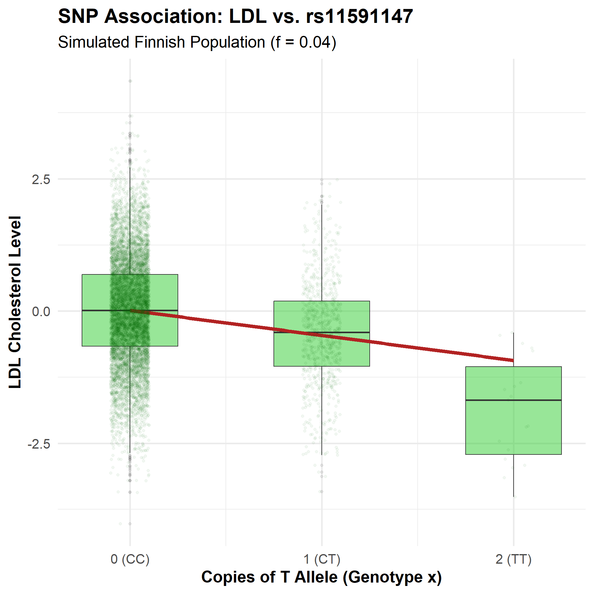
The Additive Model
We fit a linear regression: \[y = \mu + x\beta + \varepsilon\]
Interpretation

The Interpretation
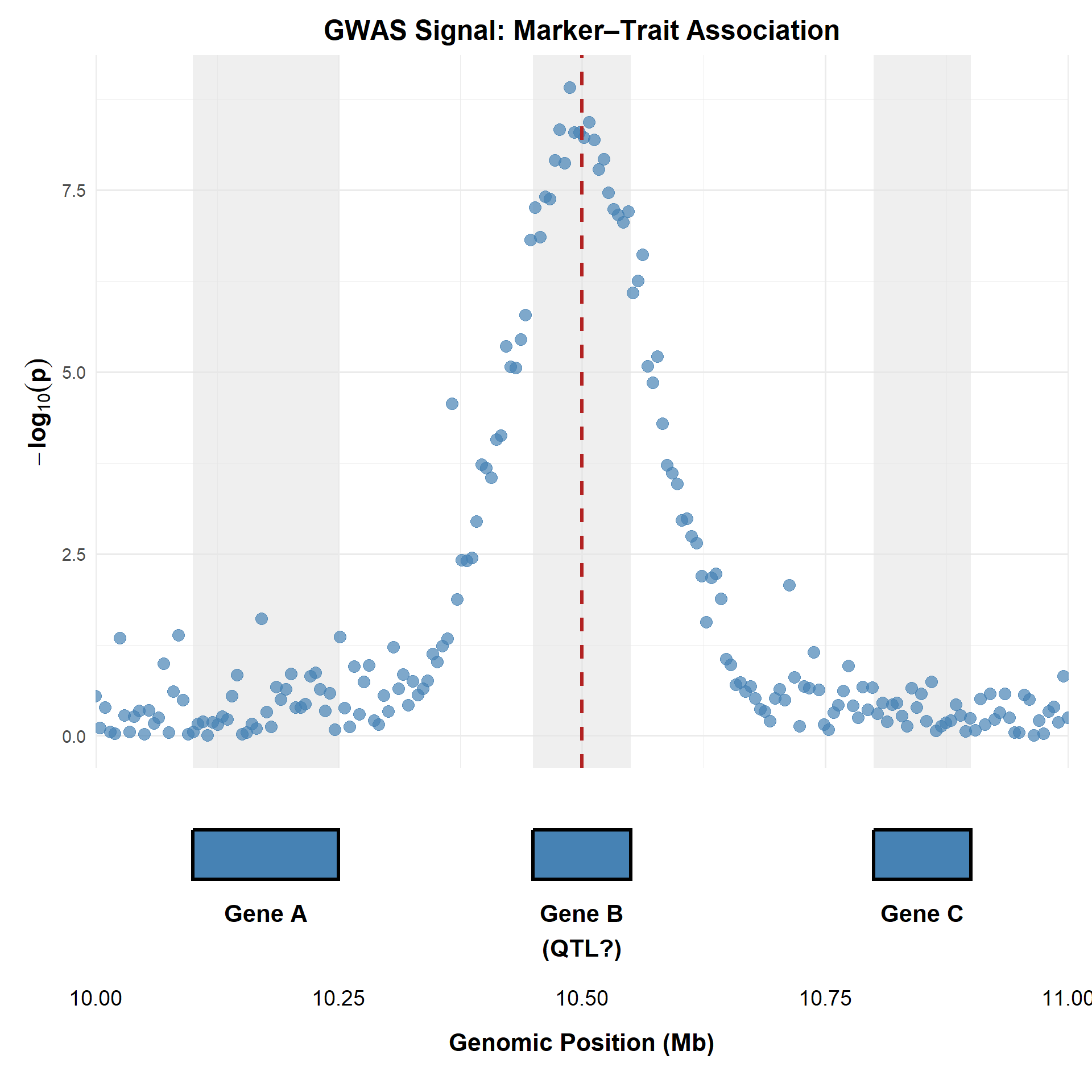
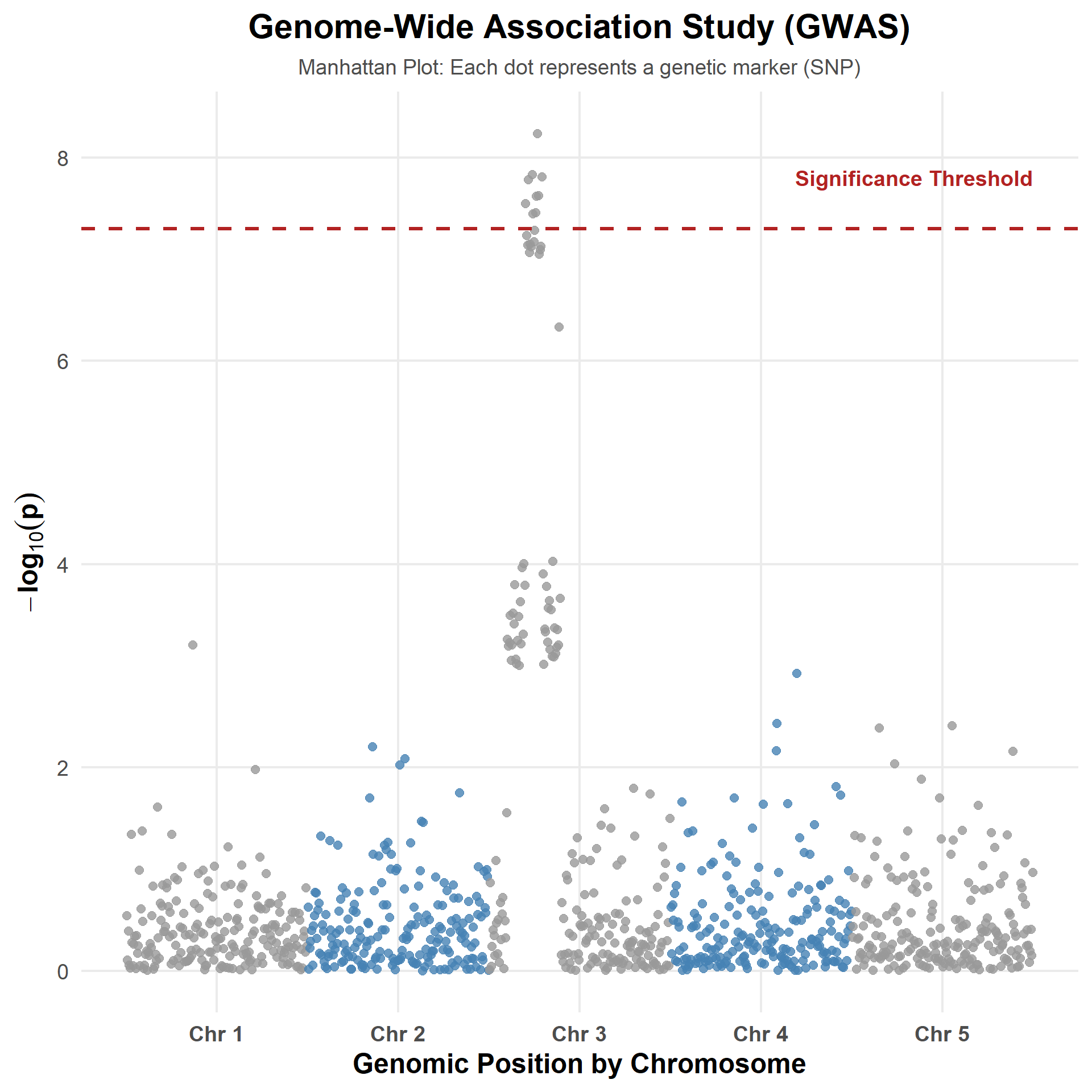
Key point This visual demonstrates Fine-Mapping: the process of narrowing down a broad GWAS “skyscraper” to the specific gene region most likely to contain the causal variant.

Each point = one SNP
Higher points = stronger evidence
against the null hypothesis.
Dashed line
Peaks indicate genomic regions
associated with the trait.

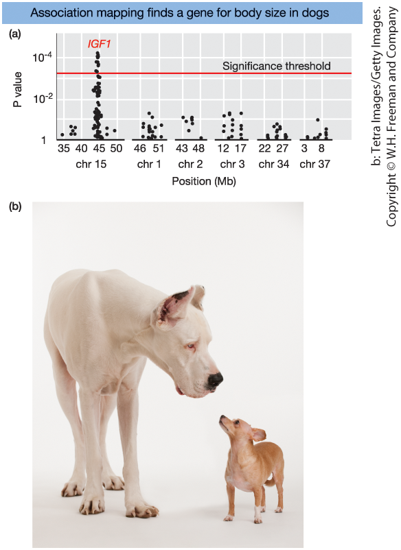
Figure 19-18.
→ Region contains the IGF1 gene
IGF1 is a major contributor to size differences.

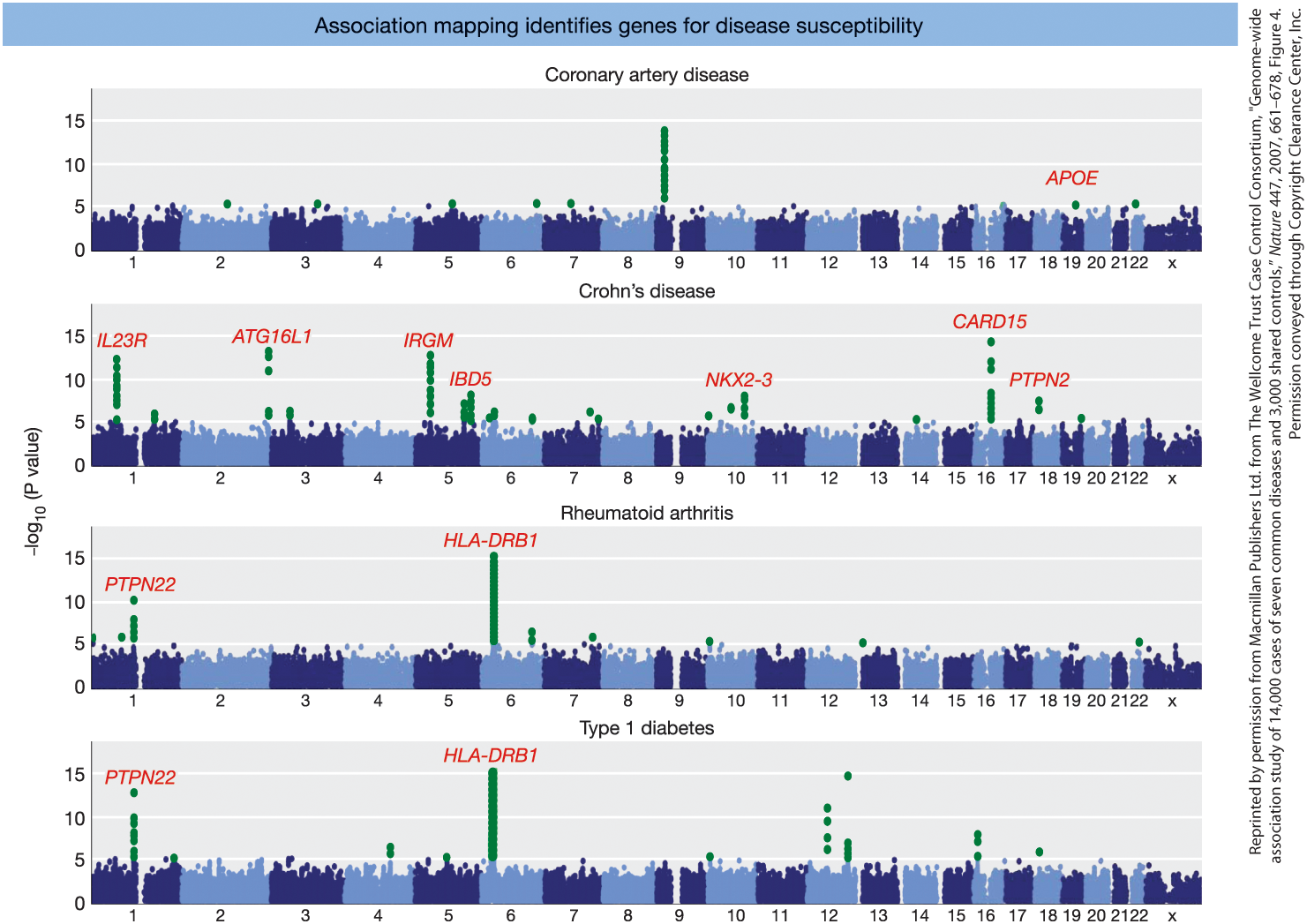
Figure 19-19.
Genome-wide association studies (GWAS)
for several common human diseases.
Examples:
What is studied?
Examples:
Core model
\[ P = G + E \]
Why it matters
Genetic Model
Genetic deviation:
\[ G = A + D \]
Only additive effects are predictably transmitted
from parents to offspring.
Additive variance (\(V_A\)) is the key component for long-term genetic change.
Breeder’s Equation
Response to selection:
\[ R = h^2 S \]
Response depends on:
High \(h^2\) → rapid response
Low \(h^2\) → limited response
Phenotype model \[ P = \mu + G + E \]
Phenotypic variance \[ V_P = V_G + V_E \]
Broad-sense heritability \[ H^2 = \frac{V_G}{V_P} \]
Narrow-sense heritability \[ h^2 = \frac{V_A}{V_P} \]
Interpretation
Total variation can be partitioned into Genetic variance and Environmental variance
Broad-sense heritability (H²)
Proportion of total variation due to genetic effects
(additive, dominance, epistatic).
Narrow-sense heritability (h²)
Proportion due to additive (transmissible) variation.
Only additive variance predicts response to selection.
The Goal of Mapping
The Strategy: GWAS
Key Discoveries from GWAS
The Result: Manhattan Plot