From GWAS results to fine-mapping and colocalisation
The workflow
There are two routes. A saved individual-level BED gbayes::gbayes() fit can be interpreted by region using LD from the same people and markers. This reuses the global posterior and does not refit it. Alternatively, start with aligned GWAS results and a Glist augmented with sparse LD. Prepare the statistics, fit each region and trait, inspect marker support, then compare fitted multi-effect components with gmap_coloc_components().
This example requires development installations of gbase, gbayes, gmap and gsim. The website displays saved results and does not run models. The current calls are shown below; a refreshed end-to-end script remains separate work.
Familiar summary-statistic calls
For statistics computed from the selected BED people, regional BayesC/BayesR can use full LD directly in memory:
G <- gbase::gprep(bedfiles="cohort.bed")
sets <- list(locus=c("marker1", "marker2", "marker3"))
fit <- gmap::gmap(Glist=G, stat=stat, sets=sets, method="bayesC",
  algorithm="mcmc", nit=1000, nburn=100, seed=10, output="full")
head(fit$stat)       # bm: native posterior effect mean; dm: PIP
head(fit$post)      # one row per region: ve, vg, vb, pi, pip, marker/range summaries
head(fit$conv)      # native R-hat, ESS, MCSE and diagnostic statuses by region
fit$cs              # marginal-PIP/LD groups by region
fit$timings         # decoding, LD product, preparation and sampling phases
gbase::mapSets(sets, Glist=G) maps named marker sets to prepared marker IDs or indices; unknown members are dropped and empty sets stay visible. gbase::getLD(G, rsids=sets$locus) returns full regional correlation in requested marker order without writing an LD file. Missing dosages are mean-imputed. Local nthreads controls decoding; the dense product uses R’s configured BLAS.
algorithm="mcmc" requires positive-definite LD, applies no PSD repair or truncation, and does not require sparse LD. algorithm="mcmc-eigen" retains the sparse-LD eigen route and its explicit retained-mass controls. Existing regions and score/information calls retain their advanced defaults.
Familiar calls default to one chain, 1000 post-burn sweeps, 100 burn-in sweeps, h2=.5, mc=5000, BayesC weights c(.99,.01), and learned slab/residual variances and mixture weights. Residual learning asserts in-sample LD and rejects a likelihood dimension exceeding the selected reference sample count. nit, nburn, nthin, nrun, seed, pi, gamma, vb, ve and updateB/updateE/updatePi adapt to native controls; conflicting explicit aliases and nested settings are rejected. post$vg is the posterior mean of the joint-effect quadratic b' C b / n, evaluated from the sampler’s cached residual; it is not qgg’s separate genetic-variance hyperparameter draw. post$pi is the total non-null mixture probability, pi0, pi1, … retain each mixture weight, and post$pip sums marker PIPs (expected active count). conv has rhat_*, ess_*, mcse_* and status_* columns for these quantities; these are native diagnostics, rather than qgg Geweke z scores. Fixed quantities, missing traces and single-chain limitations remain explicit. ntrials and cutoff record selected eigen attempts and retained mass. One-chain fits remain provisional. Original native tables and details remain available.
BayesC/BayesR accept the same optional LD-swap controls as gbayes() on both dense and eigen routes:
fit <- gmap::gmap(Glist=G, stat=stat, sets=sets, method="bayesC",
  algorithm="mcmc", nit=1000, nburn=100, nrun=4, seed=10,
  control=list(ld_swap=list(probability=.05, minimum_r2=.8,
    maximum_friends=50L, moves=1L)))
fit$ld_swap
The sampler proposes relocating an active effect to an inactive LD neighbour, using its native Metropolis-Hastings acceptance rule. probability selects a sweep for up to moves proposals; minimum_r2 and maximum_friends bound the neighbour list. LD is defined by the fitted cross-products, including retained eigen truncation. The result has one row per selected region/trait fit, with attempted and accepted counts and an acceptance rate; per-chain counts are in details. Counts include burn-in. Without an attempted move the rate is NA. These counts describe proposal activity, not convergence. The native neighbour list is prepared once per region/trait likelihood and shared across its chains; LD is not recomputed from genotypes for each swap.
Probability defaults to zero in both packages; zero moves also disables swaps and neighbour preparation. Optional neighbour preparation adds cost, particularly for eigen operators. Existing manuscript timings used swaps disabled and are preserved. The multi-effect variational method does not accept LD-swap controls.
Saved regional or genome-wide PIPs can be grouped without refitting:
groups <- gmap::getCredibleSets(Glist=G, fit=fit, sets=sets,
  cs_threshold=.8, cs_r2=.5, cs_method="CS2")
This standalone native helper reproduces qgg CS2/CS3 ordering and strict LD^2 > r2 neighborhoods. Its grouping target is marginal-PIP mass (expected active-marker count), not guaranteed component credible coverage. It has no qgg runtime dependency. Multi-trait results require an explicit trait.
From an individual-level BED fit to regional marker support
First fit the whole selected marker panel using pre-adjusted phenotypes, as in the Bayesian regression guide. Then prepare sparse LD from that same Glist and use it to interpret the saved posterior in named regions:
G <- gbase::gprep(bedfiles="cohort.bed", ids=phenotypes$id)
fit <- gbayes::gbayes(data=phenotypes, Glist=G, trait="height", method="bayesr",
  prior=list(residual_variance=.8, effect_variance=.2),
  control=list(burnin=1000, sampling_sweeps=4000, seeds=c(31,97)))

G <- gbase::gprep(Glist=G, task="sparseld", out_prefix="build/ld/cohort",
  r2=0, max_distance_bp=0, max_distance_variants=49)
regions <- list(locus=G$sparseLD$marker_metadata$marker_id[101:150])
mapped <- gmap::gmap_bed(fit, G, regions)
summary(mapped)
plot(mapped, region="locus", trait="height")
The 101:150 marker range is illustrative; choose a biological region in reference order. Here r2=0 and the 49-marker window retain every pair in that contiguous 50-marker region. Set the window to span the largest region you intend to interpret. gmap_bed() checks the saved fit against the Glist’s selected people, physical BED marker offsets, alleles and frequencies. It rejects incomplete within-region LD unless control=list(allow_incomplete_ld=TRUE) is explicitly supplied; those groups are then labelled approximate. Regions are bounded to 2048 markers by default.
The returned PIPs and effect summaries are from the global BED fit. Native gmap groups these marginal PIPs using within-region LD. These groups are not component credible sets, do not carry guaranteed coverage and are not regional refits. Inspect chain behavior and parameter summaries on fit itself. The same call accepts a saved joint-trait BED BayesC/BayesR fit and returns separate labelled regional views for each trait.
Prepare summary statistics
Each trait has an ordinary data frame with marker, allele1, allele2, beta, se and n. allele1 is the effect/counting allele. Marker rows and alleles must already match the entire reference in order. Alignment is a separate task; this helper never flips, reorders or drops markers.
library(gmap)
G <- readRDS("build/examples/gmap-workflow/Glist.rds")
example <- readRDS("build/examples/gmap-workflow/workflow.rds")
gwas <- example$gwas
head(gwas$A)
stat <- gmap_stat(gwas, G,
                 phenotype_variance = example$phenotype_variance)
regions <- example$regions
The helper supports continuous outcomes analysed by ordinary linear regression with an intercept and conventional standard errors: a separate y ~ marker regression for each marker, without other covariates. All markers within a trait must use the same individuals. Supply the sample phenotype variance, not the residual variance or an assumed value of one.
For centered genotype \(x_j\) and outcome \(y\), the OLS identities give:
\[ d_j=x_j^\mathsf{T}x_j = \frac{(n-1)s_y^2}{(n-2)\operatorname{SE}(\hat\beta_j)^2+\hat\beta_j^2}, \qquad x_j^\mathsf{T}y=d_j\hat\beta_j. \]
gmap_stat() returns marker_ss = d and score = d * beta. The native model combines these with the regional LD correlation matrix \(R\):
\[ X^\mathsf{T}X \approx D^{1/2} R D^{1/2},\qquad D=\operatorname{diag}(d_j). \]
The marginal conversion is exact under the stated OLS contract. The full matrix is exact only with matching in-sample LD, apart from storage precision. This example uses an independent panel, so its off-diagonal entries are approximations. The SuSiE summary-statistic documentation also explains the role of in-sample LD in recovering an individual-data fit.
Covariate-adjusted, mixed-model, logistic, robust-SE, meta-analysis and varying-sample-size summaries are outside this helper’s contract. It cannot recognise the generating analysis from numbers alone. Supplying equal n does not prove identical samples. Correctly prepared cross-products can still be passed directly to gmap(); z-only conversion is deferred.
A small simulation with known truth
The complete script generates binomial dosages with correlated neighbours and uses gsim() for continuous phenotypes. The artificial coordinates have no biological interpretation.
| Setting | Value |
|---|---|
| GWAS cohorts | Two disjoint cohorts of 10,000 individuals each |
| LD reference | Independent 4,000-individual panel from the same generator |
| Regions | Two artificial chromosomes, 20 markers each |
| Genotype construction | Allele frequency 0.3; adjacent copy probability 0.8 |
| Shared region | m08 affects both traits |
| Distinct region | m25 affects A; m36 affects B |
| Effects | 0.12 and 0.14 per standardized dosage; converted to raw-dosage units |
| Residual variance | Known simulation value 1, fixed during fitting |
| Seeds | Genotypes 20260915; gsim 20260916 and 20260917 |
The LD reference retains all within-region correlations, is prepared once, and caches one eigensystem per region. Each call reuses that preparation across traits. The script fits traits separately; it is not a joint multivariate Bayesian model. Marginal GWAS results are calculated separately in each cohort.
By default, gmap() first retains 99.5% of the positive regional LD eigenvalue mass, then tries 99% and 95% only when the earlier likelihood does not meet the method’s convergence rule. The eigendecomposition is not repeated. For a region with several traits, one threshold is accepted only when every trait passes. Multi-effect fits use their native convergence flag; BayesC and BayesR use the configured maximum between-chain PIP range. The selected threshold, achieved mass, retained rank and score-projection change are in diagnostic_summary; eigen_attempts retains one lightweight row per attempted trait and threshold.
fit$diagnostic_summary
fit$eigen_attempts

# Exact full-rank likelihood, without fallback
full <- gmap(stat, G, regions, method = "multi_effect", prior = prior,
  control = list(effects = 3,
                 eigen = list(retained_positive_mass = 1)))
If no attempted likelihood passes, the last complete fit is returned with status = "provisional" and a warning; the threshold is therefore never hidden. Only positive directions are retained, materially indefinite LD is rejected, and every truncated likelihood explicitly projects the score into the retained space. Residual-variance learning currently requires the full-rank setting.
Fit the three methods
prior <- list(residual_variance = 1, effect_variance = .04)
mc <- list(burnin = 1000, sampling_sweeps = 5000,
           seeds = c(31, 97), retain_diagnostics = TRUE)

bayesc <- gmap(stat, G, regions, method = "bayesc",
  prior = c(prior, list(inclusion_probability = .05)), control = mc)
bayesr <- gmap(stat, G, regions, method = "bayesr",
  prior = c(prior, list(weights = c(.95, .01, .01, .03))), control = mc)
multi <- gmap(stat, G, regions, method = "multi_effect", prior = prior,
  control = list(effects = 3, max_sweeps = 500,
                 estimate_effect_variance = TRUE,
                 eigen = list(retained_positive_mass = 1)))
These deliberately specified priors differ between methods; the example is not a ranking experiment. effect_variance is on the original GWAS effect scale. BayesR uses its default variance multipliers. Multi-effect can reduce unneeded component variances to zero. Residual variance is fixed in this example; the known simulation value is not a general recommendation for data. A regional fit also omits the other region’s small genetic contribution, so fixing the residual variance at one is a deliberate working approximation. The multi-effect fit uses full rank because its saved components are used for colocalisation below; component colocalisation does not accept a truncated likelihood.
Learn parameters when needed
The default keeps the supplied variances and mixture weights fixed. To learn BayesC/BayesR effect variance and mixture weights, enable the native updates and supply explicit hyperpriors. For example, using the external-panel inputs above:
learned <- gmap(stat, G, regions, method = "bayesr",
  prior = list(residual_variance = 1, effect_variance = .04,
               effect_variance_prior = list(df = 6, scale = .04),
               weight_prior = c(95, 1, 1, 3)),
  control = c(mc, list(estimate_effect_variance = TRUE,
                      estimate_weights = TRUE)))
learned$parameters
These hyperpriors illustrate the syntax; they are not universal settings. The variance prior is scaled inverse chi-square (df, scale), and scale is not its mean. weight_prior contains Dirichlet concentrations, null component first. BayesR variance multipliers remain fixed. The parameter table distinguishes fixed values from pooled MCMC posterior means or multi-effect variational estimates. Per-chain parameter means and optional traces remain in details.
Residual learning needs in-sample LD, so it is not enabled for this example’s independent reference panel. With a separately prepared complete G_in_sample and statistics from the same individuals and centered design, the pattern is:
# Template: y, stat_in_sample and G_in_sample must describe the same data.
normalization <- list(A = list(response_ss = sum((y - mean(y))^2),
                               likelihood_dimension = length(y) - 1,
                               in_sample_ld = TRUE))
learned_multi <- gmap(list(A = stat_in_sample), G_in_sample, regions,
  method = "multi_effect", prior = prior,
  control = list(effects = 3, estimate_effect_variance = TRUE,
                 estimate_residual_variance = TRUE),
  normalization = normalization)
learned_multi$parameters
For an intercept-only model the likelihood dimension is n - 1, not the n - 2 used by each marginal regression’s standard error. Covariate-adjusted inputs require the corresponding residualized design and response. The function cannot verify sample identity; in_sample_ld=TRUE is an explicit assertion. Thresholded or incomplete regional LD is rejected for residual learning, and control$eigen$retained_positive_mass must be 1.
BayesC/BayesR additionally require residual_variance_prior = list(df=..., scale=...) when estimate_residual_variance=TRUE. Multi-effect uses variational updates without that hyperprior and reports its residual trace and convergence flag. Normalization applies to every selected region for its trait. A regional residual includes effects omitted from that region; it is not automatically the whole-genome environmental variance. Subsequent colocalisation uses fitted parameter values, without integrating parameter uncertainty.
Inspect estimates, sets and chains
summary(bayesr)
head(bayesr$estimates)
posterior_sets <- gmap_sets(bayesr)
posterior_sets$summary
posterior_sets$members
gmap_bfdr(bayesr, threshold = c(0.8, 0.9, 0.95))
gmap_bfdr(bayesr, target = 0.05)
bayesr$details$shared$A$chain_agreement
plot(bayesr, region = "shared", trait = "A", quantity = "chains")
summary(multi)
multi$sets$shared$A
plot(multi, region = "shared", trait = "A", quantity = "objective")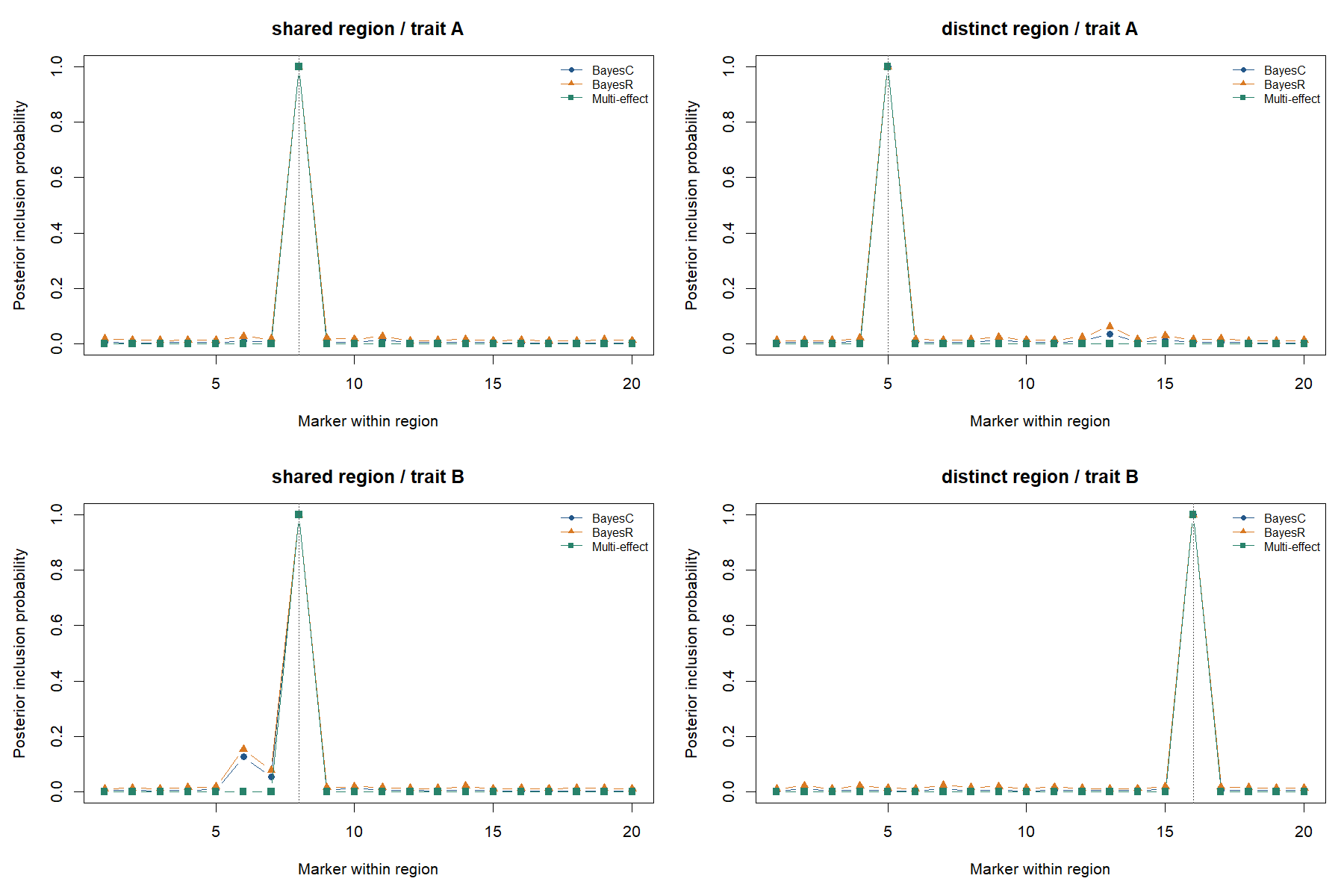
For this fixed simulation, all methods selected the causal marker first:
| Region / trait | Top marker (all methods) | BayesC sum of PIPs | BayesR sum of PIPs | Multi-effect sum of PIPs |
|---|---|---|---|---|
| Shared / A | m08 | 1.109 | 1.297 | 1.000 |
| Shared / B | m08 | 1.273 | 1.465 | 1.000 |
| Distinct / A | m25 | 1.155 | 1.356 | 1.000 |
| Distinct / B | m36 | 1.111 | 1.293 | 1.000 |
The top-marker PIPs exceed 0.99999. Each fit returned one complete set. All four multi-effect fits converged in two sweeps. The largest BayesR PIP range between the two chains was 0.014. These strong signals make an easy workflow demonstration, not a demanding fine-mapping evaluation.
BayesC/BayesR report PIPs pooled over the two chains. Chain-specific PIPs and ranges are available; agreement alone does not certify convergence. Their sets group marginal PIP mass within LD neighbourhoods. Multi-effect sets represent component assignment probabilities. These set probabilities are not interchangeable, and this one simulation does not establish coverage. The sum of PIPs is the expected number of active markers, not necessarily the number of independent signals.
gmap_sets() keeps the native interpretation in its meaning column: marginal_pip_mass for BayesC/BayesR neighbourhood groups and component_assignment for multi-effect credible sets. Its summary table also retains completeness, pairwise LD purity, incomplete-LD, duplicate and fit-status fields. The member table gives the markers, posterior weights and LD to the lead.
gmap_bfdr() uses only marker PIPs. At threshold \(t\), its expected number of false discoveries is \(\sum_{j:PIP_j\ge t}(1-PIP_j)\) and BFDR is that value divided by the number selected. With target, it returns the largest marker group defined by a PIP threshold whose BFDR is no larger than the target. This posterior summary does not provide a frequentist FDR guarantee.
Compare the traits without refitting
shared <- gmap_coloc_components(
  multi, multi, G, trait1 = "A", trait2 = "B",
  control = list(complete_region_coverage = TRUE,
                 non_overlapping_samples = TRUE)
)
summary(shared)
shared$estimates
shared$component_status
plot(shared, region = "shared")
plot(shared, region = "distinct")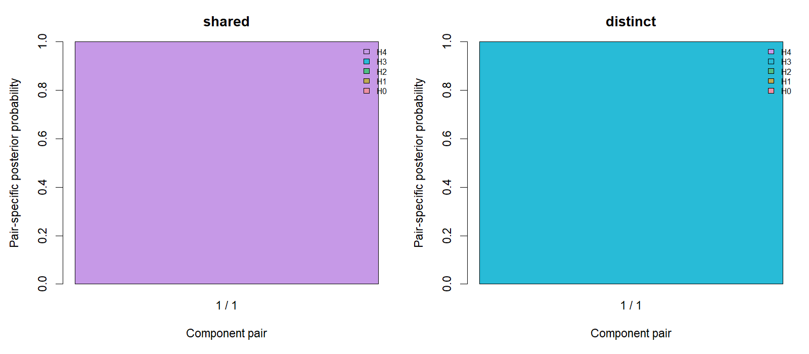
H0 means neither trait is associated; H1/H2 mean only one is associated; H3 means distinct causal variants; H4 means a shared causal variant. These are component-pair probabilities, not a single region-wide posterior. The defaults are per-variant priors \(p_1=p_2=10^{-4}\) and \(p_{12}=10^{-5}\). In this run, shared-region H4 was 0.999999999991; distinct-region H3 rounded to 1, with H4 about \(3.24\times10^{-45}\). These values reflect this strong, artificial example and its specified priors, not general performance. Changing these priors reuses the saved evidence. No eligible component pairs means there is no eligible comparison; it is not evidence for H0.
Numerical checks and saved results
The script compares the converted scores and diagonals against direct cross-products from the simulated individuals. It also fits all three methods from both routes, with the same LD and seeds, and checks PIPs and posterior means. That validates the conversion; it does not validate the external-LD approximation or establish calibration. The LD file checksums are checked before and after fitting.
The run on 15 September 2026 used gsuite 0.43.0, gsim 0.9.0 and R 4.4.1. The largest score/diagonal discrepancy was \(1.82\times10^{-12}\); the largest posterior-mean discrepancy was \(1.11\times10^{-16}\). PIPs agreed to numerical precision. Approximate observed times for four region/trait fits per method were 0.69 s (BayesC), 6.16 s (BayesR) and 0.36 s (multi-effect). The whole script took 17.91 s, including preparation, repeat fits for verification, colocalisation and figures. These are illustrative elapsed times on one laptop, not a benchmark; another package-build process was also active.
example$conversion
example$equivalence
example$timing
summary(example$fits$bayesr)
summary(example$coloc)
workflow.rds contains the summaries, prepared statistics, truth, fitted objects and checks. report.txt records summaries and package versions. The directory also contains two figures and compact CSV tables. Saved fits can be plotted without the LD files; a new gmap_coloc_components() call requires the reference files so that eligibility and reference checks can run.
ABF colocalisation
For at most one causal variant per trait, compare the aligned GWAS tables directly. This route uses native gmap ABFs; it does not require an LD object, gmap_stat() or a Bayesian fine-mapping fit. The example’s two cohorts are disjoint, and each selected region contains one generating causal variant per trait, so it is suitable for illustrating this model.
markers <- regions$shared
first <- gwas$A[match(markers, gwas$A$marker), ]
second <- gwas$B[match(markers, gwas$B$marker), ]
abf <- gmap_coloc(
  first, second, region = "shared",
  phenotype_sd1 = sqrt(example$phenotype_variance[["A"]]),
  phenotype_sd2 = sqrt(example$phenotype_variance[["B"]]),
  p1 = 1e-4, p2 = 1e-4, p12 = 1e-5)
abf$shared_variant_probability
Each table requires rsids, chr, pos, ea, nea, b and seb. Rows and alleles must match exactly. ea is the effect allele; effects and standard errors are on the phenotype scale per allele. Phenotype standard deviations are supplied here, unlike the variances passed to gmap_stat(). The effect-prior SD is the specified fraction of each phenotype SD. Binary/log-odds, z-only and p-value-only inputs are not supported, and phenotype SD is never inferred.
H0 means neither trait is associated, H1/H2 one trait alone, H3 distinct causal variants and H4 a shared causal variant. Here these are regional probabilities under the single-causal model. The earlier multi-effect results instead apply to individual component pairs; they must not be added into a regional posterior. Marker probabilities are conditional on H4, not marginal fine-mapping PIPs.
Use separate calls to examine alternative association priors. Regional coverage and sample independence are scientific assumptions of this model and must be established by the caller. Selected MR instruments alone do not provide complete regional data. Evidence for shared association is not by itself evidence for a causal effect of one trait on another.