Bayesian genomic regression with gbayes

Fit BayesC, inspect posterior diagnostics and carry marker weights into prediction.

gbayes fits marker effects from aligned summary statistics and the shared Glist LD reference. It also supports individual BED phenotypes, multivariate fits, annotation-informed priors and several focused summary engines. This page interprets the BayesC fit from the 20K/50K simulation; alternative calls below show other available routes without attaching the displayed BayesC numbers to them. Load statistics, reference_Glist, Y and panel from the linked study overview and gbase preparation, or run the complete driver there to regenerate the saved fit.

Fit one summary trait

Trait A contributes 6,000 GWAS individuals. Its aligned table has effect estimates b, standard errors seb and sample size n for every marker. The fixed BayesC prior used in the saved run expects roughly 2% of markers to be active.

library(gbayes)

prior <- list(
  residual_variance = 1,
  effect_variance = 0.3 / (50000 * 0.02),
  inclusion_probability = 0.02
)
control <- list(
  burnin = 500L,
  sampling_sweeps = 700L,
  seeds = c(11, 29, 47, 71),
  threads = 4,
  residual_policy = "fixed"
)

fit <- gbayes(statistics$A, reference_Glist,
  method = "bayesc", trait = "A",
  prior = prior, control = control)

The fit returns one row per marker in fit$estimates, a portable allele-labelled fit$weights table, posterior parameter summaries and chain diagnostics. These are the saved parameter summaries:

Parameter	Mean	Sd	Lower	Upper	R-hat	ESS bulk
residual_variance	1	0	1	1
effect_variance	3.000e-04	0	3.000e-04	3.000e-04
active_markers	988	30.6	929	1,048	1	2775
weight_0	0.98	0	0.98	0.98
weight_1	0.02	0	0.02	0.02

Residual variance, effect variance and the mixture weights were fixed here, so their posterior standard deviations are zero and R-hat/ESS are blank. active_markers was sampled; its R-hat and bulk ESS are meaningful chain checks. Inspect the complete diagnostics and chain traces before treating a fit as stable:

fit$posterior
fit$diagnostics
fit$chains

Interpret marker support

mean is the posterior mean effect and pip is the posterior inclusion probability. PIP measures support for a nonzero effect under this model and prior; it is neither a GWAS p-value nor proof that one LD-correlated marker is the unique causal variant.

Marker	Position	Mean	Variance	PIP
m00050	50,000	0.131	1.033e-04	1
m00125	25,000	0.139	1.082e-04	1
m06170	70,000	0.0395	1.627e-04	0.964
m06958	58,000	-0.0378	1.844e-04	0.948
m02942	42,000	-0.0371	1.949e-04	0.935
m03380	80,000	-0.0362	2.035e-04	0.93
m45456	56,000	-0.0312	2.867e-04	0.833
m00998	98,000	0.0298	2.657e-04	0.832
m02924	24,000	0.0281	2.866e-04	0.797
m28637	37,000	0.0276	2.855e-04	0.794

Highest BayesC marker PIPs.

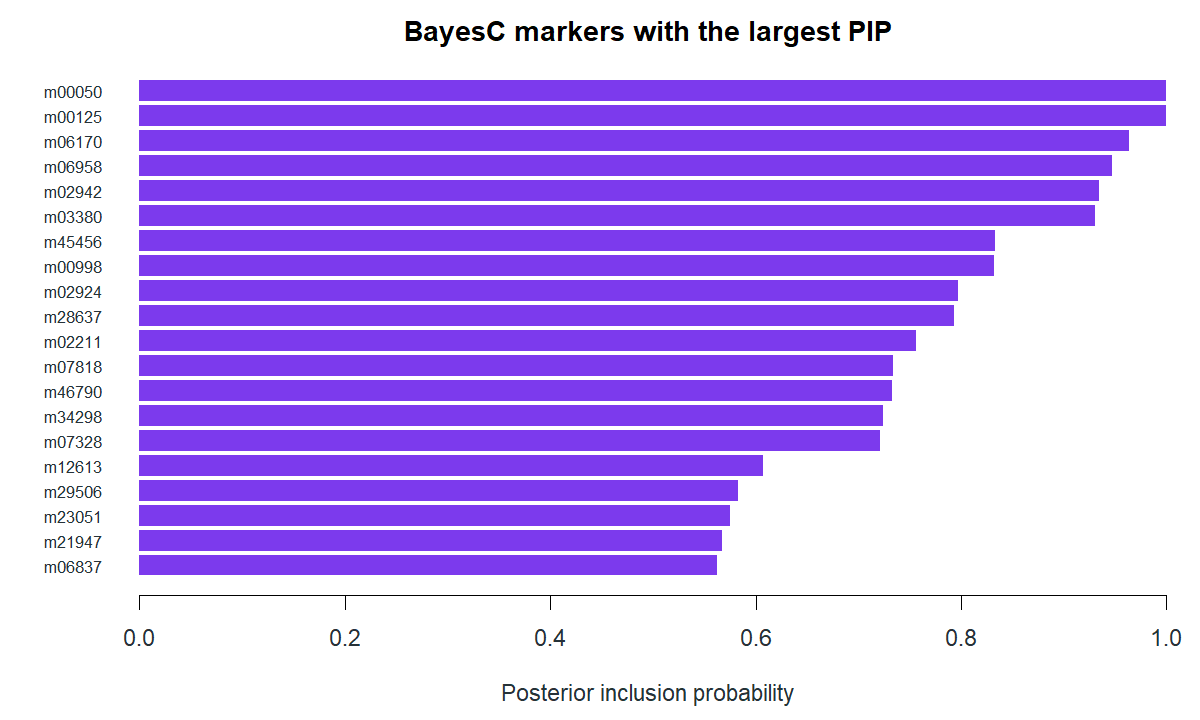
top <- fit$estimates[order(fit$estimates$pip, decreasing = TRUE), ]
head(top[c("marker", "position", "mean", "variance", "pip")], 10)
head(fit$weights)

The weights table includes marker IDs, coordinates, alleles, allele frequencies and standardized-effect columns. gscore checks these labels against a target Glist and applies the weights to held-out people.

Choose the model and data route

Route	Example call	When it is useful
Summary BayesR	gbayes(statistics$A, reference_Glist, method = "bayesr", prior = bayesr_prior)	Mixture of several nonzero effect scales.
Annotation-informed eigen blocks	gbayes(statistics$A, reference_Glist, method = "sbayesrc", annotation = component_annotation)	Verified independent LD blocks and marker annotations.
Individual-level BayesC/R	gbayes(data = phenotype_table, Glist = panel, method = "bayesc", trait = "A", prior = prior)	Fit directly to selected BED genotypes and named phenotypes.
Focused summary approximations	gbayes(statistics$A, reference_Glist, method = "variational")	Deterministic variational or shrinkage analyses with their own controls.
One regional effect	gbayes_single_effect(region_stat)	Posterior assignment probabilities under a one-effect model.

For individual-level fitting, supply a data frame with unique character id and a finite pre-adjusted phenotype column:

phenotype_table <- data.frame(id = rownames(Y), A = Y[, "A"])
bed_fit <- gbayes(data = phenotype_table, Glist = panel,
  method = "bayesc", trait = "A", prior = prior)

sbayesrc requires the verified block partition from gbase::define_ld_blocks() and a marker-aligned component annotation. Block eigensystems are prepared once per fit and reused by its chains. The Bayesian workflow guide gives the full annotation structure and describes BayesR, BayesS scaling, multivariate traits, study-specific references and method-specific approximation controls.

Continue or request posterior quantities

Long chains can resume from an exact saved continuation state when the model definition and marker order are unchanged. posterior can request genetic covariance/correlation from a declared LD reference, heritability with an explicit phenotype variance, marker partitions or predictions for selected individuals with posterior uncertainty.

fit_with_quantities <- gbayes(statistics$A, reference_Glist,
  method = "bayesc", trait = "A", prior = prior, control = control,
  posterior = list(reference = reference_Glist,
                   phenotype_variance = c(A = 1)))

fit_with_quantities$quantities

Those quantities are separate from the fixed BayesC run displayed above; use the phenotype variance of your actual trait rather than the illustrative value in the snippet.

Download posterior summaries · download the top marker estimates