Prepare genotypes and LD with gbase

Build a Glist, filter markers, publish sparse LD and align GWAS statistics.

gbase owns the data boundary shared by the analysis packages. Its Glist records the selected samples and markers, physical BED locations, allele labels and marker summaries. When LD is requested, the same object also carries the sparse-LD identity, sample and marker provenance, and LD scores. This page uses the shared 20K/50K simulation.

Prepare the panel

Start with a SNP-major PLINK BED file and matching BIM/FAM files. gprep() infers the companion paths from the BED name. Sample IDs and marker IDs are selected by name and retain their documented Glist order.

library(gbase)

prefix <- "path/to/genotypes"  # replace with your PLINK prefix
individuals <- sprintf("id%05d", 1:20000)
marker_ids <- sprintf("m%05d", 1:50000)
reference_ids <- individuals[1:18000]
regions <- split(marker_ids,
  rep(sprintf("region%03d", 1:500), each = 100))

panel <- gprep(bedfiles = paste0(prefix, ".bed"), nthreads = 4)
reference_Glist <- gprep(bedfiles = paste0(prefix, ".bed"),
  ids = reference_ids, nthreads = 4)

stopifnot(sum(lengths(panel$rsids)) == 50000)
stopifnot(length(reference_Glist$study_ids) == 18000)

The selected-reference summaries, including allele frequencies and genotype counts, come from those 18,000 people. panel retains all 20,000 people for later association scans and held-out scoring.

Review marker quality before LD construction

gfilter() returns marker names in file order. It can screen MAF, missingness, exact Hardy–Weinberg p-values, imputation INFO when supplied, allele ambiguity, indels and the assembly-specific MHC interval. The returned names can be fed back into gprep(); filtering the Glist after building LD would leave an inconsistent reference.

retained <- gfilter(reference_Glist,
  maf = 0.01, missing = 0.05, hwe = 1e-12,
  ambiguous = TRUE, indels = TRUE, verbose = TRUE)

# For a study that applies this filter:
filtered_reference <- gprep(bedfiles = paste0(prefix, ".bed"),
  ids = reference_ids, rsids = retained, nthreads = 4)

The saved 20K/50K run used all 50,000 simulated markers in its LD resource; filtered_reference above illustrates the optional QC route and is not the source of the tables below.

Compute and reuse sparse LD

The simulation has 500 independent 100-marker regions. Its full within-region LD is retained with r2 = 0; the 100-variant window bounds the calculation. For real data, choose windows and thresholds appropriate to the intended method and report them with the reference.

dir.create("analysis", showWarnings = FALSE)
reference_Glist <- gprep(Glist = reference_Glist, task = "sparseld",
  out_prefix = "analysis/reference-LD",
  max_distance_bp = 0, max_distance_variants = 100,
  r2 = 0, block_size = 128, nthreads = 4,
  overwrite = TRUE)
reference_Glist$assembly <- "artificial-20k-50k"

block_table <- data.frame(
  block_id = names(regions),
  first_marker = vapply(regions, `[`, character(1), 1L),
  last_marker = vapply(regions, function(x) tail(x, 1L), character(1))
)
reference_Glist <- define_ld_blocks(reference_Glist, block_table)
verify_ld(reference_Glist)
saveRDS(reference_Glist, "analysis/reference-Glist.rds")

define_ld_blocks() verifies that the named, ordered partition is exhaustive and that retained LD does not cross blocks. verify_ld() explicitly scans the complete resource after construction or transfer. Routine readers use the lightweight Glist identity check when opening the same immutable LD files. Keep the Glist RDS together with its referenced LD files.

Item	Value
Individuals	20,000
Markers	50,000
Chromosomes	1
LD reference individuals	18,000
Independent LD blocks	500
Mean MAF	0.3
Mean LD score	1.97

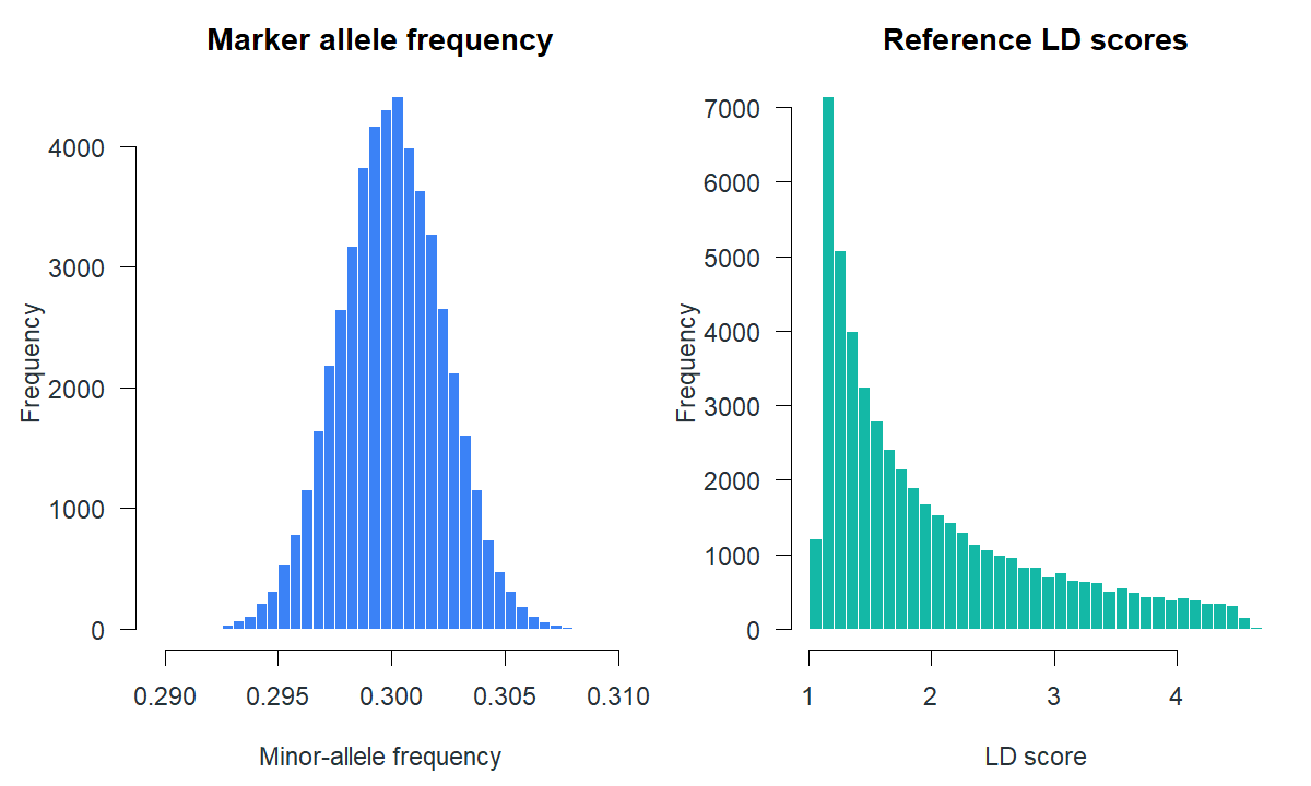
Histograms of minor-allele frequency and reference LD score across 50,000 simulated markers. — Minor-allele frequencies and LD scores from the reference.

Inspect LD and compute annotation scores

Ordinary LD scores are already stored in the Glist. ld_region() returns a named dense matrix for a small ordered marker set; ld_eigen() returns its complete verified eigensystem. Use these for inspection or methods that need a regional matrix rather than repeatedly reading the whole reference.

reference_Glist <- readRDS("analysis/reference-Glist.rds")
validate_Glist(reference_Glist)
scores <- ld_scores(reference_Glist)
R_region1 <- ld_region(reference_Glist, regions$region001)
eigen_region1 <- ld_eigen(reference_Glist, regions$region001)

ld_markers <- unlist(reference_Glist$rsidsLD, use.names = FALSE)
annotation <- matrix(as.numeric(ld_markers %in% regions$region001), ncol = 1,
  dimnames = list(ld_markers, "region001"))
annotation_scores <- ld_scores(reference_Glist, annotation = annotation)

An annotation score at marker j accumulates squared LD from j to the annotated markers, including LD crossing the annotation boundary. This is the input needed for standard stratified LDSC in gcorr.

Align GWAS statistics

checkStat() maps a reported GWAS table to the reference’s marker IDs, coordinates and effect-allele direction. It returns an ordinary data frame in reference order. In the simulated run, the following explicit options retain all 50,000 markers so the methods share the same marker universe:

aligned <- checkStat(reference_Glist, raw_stat,
  excludeMAF = NULL, excludeMAFDIFF = NULL, excludeINFO = NULL,
  excludeCGAT = FALSE, excludeINDEL = FALSE, excludeDUPS = TRUE,
  excludeMHC = FALSE, excludeMISS = NULL, excludeHWE = NULL)

head(aligned[c("rsids", "chr", "pos", "ea", "nea", "b", "seb", "p", "n")])

raw_stat is assembled from the glma association result. For a real GWAS, choose QC thresholds deliberately; do not infer alleles or sample sizes from the LD reference. The aligned table is used by gbayes, gcorr, gmap and VEGAS.

Download the reference summary