Polygenic scoring with gscore
gscore applies allele-labelled marker weights to selected people in a gbase Glist. It can produce total scores, scores for named marker sets and several weight columns in one pass. It also constructs clumping-and-thresholding (C+T) weights from aligned GWAS statistics and stored sparse LD. The shared simulation holds out 2,000 individuals for this example. Run the overview loading block first for prefix, Y, bayes_fit, gene_sets, statistics and reference_Glist.
Apply BayesC weights
The gbayes fit provides standardized, portable weights for trait A. The target Glist selects only the held-out people from the same PLINK files. sets contain marker names; the Glist resolves their BED locations and the scorer accumulates their contributions while reading the target panel.
library(gbase)
library(gscore)

holdout_ids <- sprintf("id%05d", 18001:20000)
test_Glist <- gprep(bedfiles = paste0(prefix, ".bed"),
  ids = holdout_ids, nthreads = 4)

prediction <- gscore(bayes_fit$weights, test_Glist,
  sets = gene_sets[1:20], include_total = TRUE,
  coding = "standardized", scale_scores = FALSE,
  control = list(threads = 4))

dim(prediction$scores)
colnames(prediction$scores)[1:6]
The score matrix has 2,000 rows in selected individual order. Its A column is the total BayesC score; the remaining columns are the requested gene contributions. Since scale_scores = FALSE, scores are not standardized again across the target cohort.
Evaluate the held-out score
Join scores to outcomes by individual ID, rather than relying on row position. Here the same trait A score is correlated with all three simulated outcomes; the B and C rows are cross-trait associations, not separately fitted B or C prediction models.
observed <- Y[rownames(prediction$scores), , drop = FALSE]
trait_A_score <- prediction$scores[, "A"]
vapply(colnames(observed), function(trait)
cor(trait_A_score, observed[, trait]), numeric(1))| Trait | Correlation with trait A score | Holdout individuals |
|---|---|---|
| A | 0.305 | 2,000 |
| B | 0.185 | 2,000 |
| C | 0.179 | 2,000 |
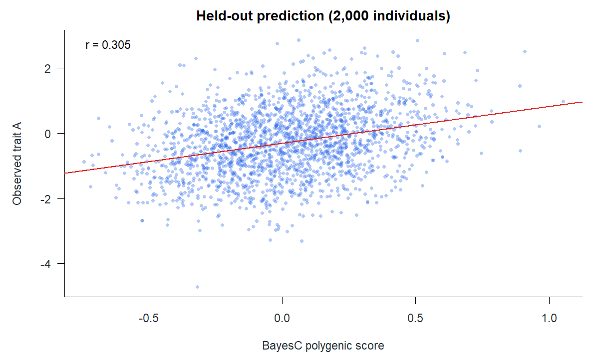
The 0.305 correlation is descriptive for one simulated holdout. Assess score calibration and transport separately when applying weights to another cohort.
Inspect marker and set coverage
gscore() checks marker IDs, coordinates and effect/other alleles. It handles exact and swapped allele orientation and records unmatched markers. Review these before interpreting a score, especially after moving weights between cohorts.
prediction$alignment
head(prediction$coverage)
prediction$missing_set_markers
The first six sets in this same-panel holdout all had complete marker coverage:
| Set | Requested markers | Used markers | Missing from Glist | Missing from weights |
|---|---|---|---|---|
| gene0001 | 21 | 21 | 0 | 0 |
| gene0002 | 79 | 79 | 0 | 0 |
| gene0003 | 22 | 22 | 0 | 0 |
| gene0004 | 78 | 78 | 0 | 0 |
| gene0005 | 23 | 23 | 0 | 0 |
| gene0006 | 77 | 77 | 0 | 0 |
control = list(missing_markers = "error") makes a missing weighted marker fatal; the default records and drops it. Use that stricter setting when the expected target marker universe should match exactly.
Construct another score from GWAS evidence
clump_threshold() chooses markers by GWAS p-value, LD and distance. It needs an LD resource retaining every pair its requested window could inspect. The main tutorial reference has a 100-variant construction limit, so it cannot be used for a 250 kb C+T window even on this artificial panel. Construct a separate clumping reference with no variant-count limit and a base-pair window at least as wide as the clumping rule:
dir.create("analysis", showWarnings = FALSE)
ct_reference <- gprep(bedfiles = paste0(prefix, ".bed"),
  ids = sprintf("id%05d", 1:18000), nthreads = 4)
ct_reference <- gprep(Glist = ct_reference, task = "sparseld",
  out_prefix = "analysis/clumping-LD",
  max_distance_bp = 250000, max_distance_variants = 0,
  r2 = 0.1, block_size = 128, nthreads = 4)

ct_weights <- clump_threshold(statistics$A, ct_reference,
  p_threshold = 5e-8, r2_threshold = 0.1,
  window_bp = 250000)

ct_prediction <- gscore(ct_weights, test_Glist,
  coding = "standardized", scale_scores = FALSE,
  control = list(threads = 4))
This C+T call is a supported alternative; the displayed scatter and correlations use BayesC weights only. C+T needs the aligned b, seb, p and n fields. Save ct_reference with its LD files for reuse; the clumping resource does not need to be recomputed for each trait.
Score shape and coding choices
| Capability | How to request it | What to inspect |
|---|---|---|
| Several scores at once | Add numeric weight columns to one allele-labelled weight table. | prediction$scores has one column per score. |
| Gene or other marker sets | Supply named marker vectors through sets. |
coverage, set_membership and missing_set_markers. |
| Weighted set totals | Supply set_weights named exactly like sets. |
Confirm the intended multipliers in coverage. |
| Raw mean-imputed coding | Set coding = "raw_mean_imputed" for weights defined on raw dosage. |
Coding and allele-frequency provenance. |
| Cohort-standardized outputs | Set scale_scores = TRUE. |
Scaling changes the reported score units. |
The public interface also exposes the lower-level gscore_bed() for a caller that already has physical BED indices and coefficient matrices. Most users should pass a Glist to retain identity and allele checks. See the scoring guide for the weight contract.
Download prediction metrics · download all set-coverage rows