Heritability and genetic correlation with gcorr

Estimate genome-wide, partitioned and regional genetic relationships from GWAS summaries.

gcorr works with aligned summary statistics. The convenient ldsc() route uses LD scores and reference metadata already held by a gbase Glist. Other public functions provide GNOVA, SumHer, regional covariance methods, covariance models and Mendelian randomisation when their additional inputs are available. This page uses the three disjoint GWAS cohorts from the shared simulation. Run the overview’s loading block first for statistics, reference_Glist and regions.

Estimate genome-wide quantities

statistics is a named list of aligned A, B and C tables from glma. The traits use the same reference markers in the same order. The disjoint GWAS cohorts justify a zero cross-trait overlap intercept in this simulated example; that assumption must be reconsidered for overlapping cohorts.

library(gcorr)

ordinary <- ldsc(statistics, reference_Glist,
  what = "rg", block_count = 200L,
  overlap_intercept = 0,
  marginal_intercept = "fixed_one")

ordinary$estimates
ordinary$h2
ordinary$rg

The h2 rows estimate SNP heritability; rg rows estimate the correlation between genetic effects for trait pairs. The reported standard errors use contiguous delete-block jackknife calculations.

Quantity	Trait1	Trait2	Estimate	Standard error	P value
h2	A		0.267	0.0551	1.291e-06
h2	B		0.303	0.0646	2.660e-06
h2	C		0.246	0.0667	2.223e-04
rg	A	B	0.669	0.142	2.331e-06
rg	A	C	0.613	0.155	7.285e-05
rg	B	C	0.749	0.138	6.110e-08

Genetic-correlation matrix for A, B and C.

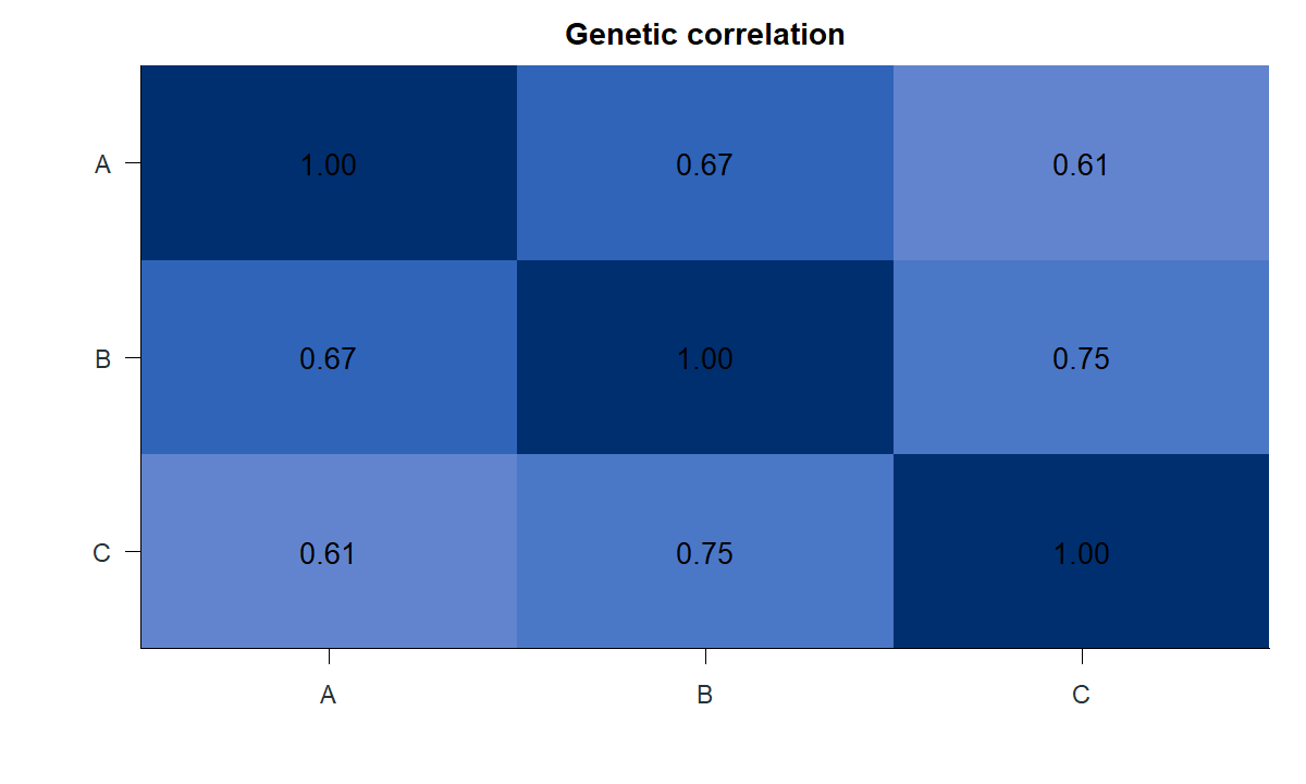
In this one run, the estimated genetic correlations lie between about 0.61 and 0.75. A correlation describes shared genetic effects on the model’s scale; it does not establish a causal relationship between traits. The uncertainty procedure has focused validation limits, so inspect diagnostics and avoid presenting these intervals as fully calibrated for every study.

Attribute heritability to a marker group

The first 80 artificial regions form an enriched annotation. Standard stratified LDSC computes an annotation LD-score column; at any marker it includes LD to annotated markers, including LD that crosses the annotation boundary. The residual column covers the remaining marker membership.

enriched_markers <- unlist(regions[1:80], use.names = FALSE)

partitioned <- ldsc(statistics, reference_Glist,
  sets = list(enriched = enriched_markers),
  residual = TRUE, set_model = "stratified",
  what = "rg", block_count = 200L,
  overlap_intercept = 0,
  marginal_intercept = "fixed_one")

subset(partitioned$estimates,
  trait1 == "A" & is.na(trait2) &
    quantity %in% c("h2", "enrichment"))

The trait A rows from this fit show a total h2 of about 0.36, with about 0.267 attributed to the enriched category. enrichment compares a category’s heritability share with its marker share. It is a model-based estimate, not a count of causal variants.

Component	Quantity	Estimate	Standard error	P value
all	h2	0.36	0.0695	2.139e-07
enriched	h2	0.267	0.06	8.372e-06
enriched	enrichment	4.63	0.541	1.074e-17
Residual	h2	0.0933	0.0351	0.00791
Residual	enrichment	0.308	0.103	0.0028

set_model = "grouped" is also available. It masks the existing ordinary LD-score vector by group membership and can avoid recomputing annotation scores. It answers a different grouped question because LD crossing group boundaries is not allocated to the same annotation columns:

grouped <- ldsc(statistics, reference_Glist,
  sets = list(enriched = enriched_markers), residual = TRUE,
  set_model = "grouped", what = "rg",
  block_count = 200L, overlap_intercept = 0,
  marginal_intercept = "fixed_one")

The displayed partitioned table belongs to the stratified fit, not the grouped example.

Work at regional or covariance level

One prepared regional LD object can be reused across methods and trait pairs. The preparation loads the requested regions and verifies their complete eigensystems once in the current R session:

prepared_regions <- gcorr_prepare_regions(reference_Glist,
  regions = regions[1:20])

regional_h2 <- gcorr_hess(statistics$A, prepared_regions,
  maximum_components = 0, minimum_eigenvalue = 0)
regional_h2$estimates

This call illustrates HESS; regional results were not part of the displayed LDSC table. Regional methods require method-specific sample overlap, eigenvalue and inference choices.

Analysis	Public interface	Additional information needed
Genome-wide architecture	gcorr_gnova(), gcorr_sumher()	Method-specific LD scores, tagging or annotation quantities.
Regional heritability/covariance	gcorr_hess(), gcorr_rho_hess(), gcorr_supergnova(), gcorr_lava(), gcorr_hdll()	Prepared regional LD and the method’s sampling assumptions.
Multitrait covariance models	gcorr_covariance(), gcorr_sem(), gcorr_ggm()	Labelled covariance and its sampling covariance.
Mendelian randomisation	gcorr_prepare_mr(), gcorr_gsmr(), gcorr_mr_ivw()	Harmonized instruments, signed LD and explicit exposure/outcome assumptions.

The method guide gives the exact inputs and scope for each family. ordinary$diagnostics and partitioned$diagnostics retain the fit checks and assumptions.

Download genome-wide estimates · download trait A partitioned estimates