Regional fine-mapping with gmap
gmap works at a declared set of regions rather than fitting the complete genome at once. It offers regional multi-effect, BayesC and BayesR fits, posterior sets, Bayesian FDR summaries and colocalisation. It can also interpret regions from an existing individual-level gbayes fit. This page uses the A and B summaries and the LD resource from the shared simulation. Run the overview’s loading block first for statistics, reference_Glist, Y and regions; the glma page defines the named gwas_ids.
Prepare the regional likelihood
gmap_stat() converts ordinary intercept-only linear GWAS b and seb into score and information inputs using the observed phenotype variance. It checks exact marker and allele order against the complete Glist LD reference. Provide the sample variance of the phenotype in each GWAS cohort, with R’s usual n - 1 denominator.
library(gmap)

phenotype_variance <- c(
  A = var(Y[gwas_ids$A, "A"]),
  B = var(Y[gwas_ids$B, "B"])
)
prepared <- gmap_stat(statistics[c("A", "B")], reference_Glist,
  phenotype_variance = phenotype_variance)

head(prepared$A[c("rsids", "ea", "nea", "score", "information")])
The conversion assumes ordinary linear regression with a common sample size within each trait. It is not an automatic conversion for mixed-model or logistic GWAS statistics. See the full mapping guide for the individual-level route and input checks.
Fit 20 marker-defined regions
The simulated regions each contain 100 marker names in LD-reference order. The multi-effect fit below requests one effect per region and uses a sequence of retained positive eigenvalue mass targets. If a fit needs another target, its successful target and retained rank are saved in diagnostics.
fit <- gmap(prepared, reference_Glist,
  regions = regions[1:20], method = "multi_effect",
  prior = list(residual_variance = 1, effect_variance = 0.04),
  control = list(
    effects = 1L, max_sweeps = 200L,
    eigen = list(retained_positive_mass = c(0.995, 0.99, 0.95))
  ))

head(fit$estimates[c("region", "trait", "marker", "mean", "pip")])
pip is a posterior inclusion probability. mean is the posterior mean effect in the prepared regional model. The leading markers in the saved run are:
| Region | Trait | Marker | Position | Mean | PIP |
|---|---|---|---|---|---|
| region001 | A | m00050 | 50,000 | 0.314 | 1 |
| region001 | B | m00050 | 50,000 | 0.336 | 1 |
| region002 | A | m00125 | 25,000 | 0.337 | 1 |
| region002 | B | m00175 | 75,000 | 0.382 | 1 |
| region010 | A | m00998 | 98,000 | 0.084 | 0.961 |
| region019 | B | m01817 | 17,000 | 0.0482 | 0.686 |
| region014 | B | m01325 | 25,000 | 0.0444 | 0.648 |
| region015 | B | m01477 | 77,000 | -0.0401 | 0.604 |
| region004 | A | m00315 | 15,000 | 0.0397 | 0.58 |
| region014 | A | m01371 | 71,000 | 0.039 | 0.559 |
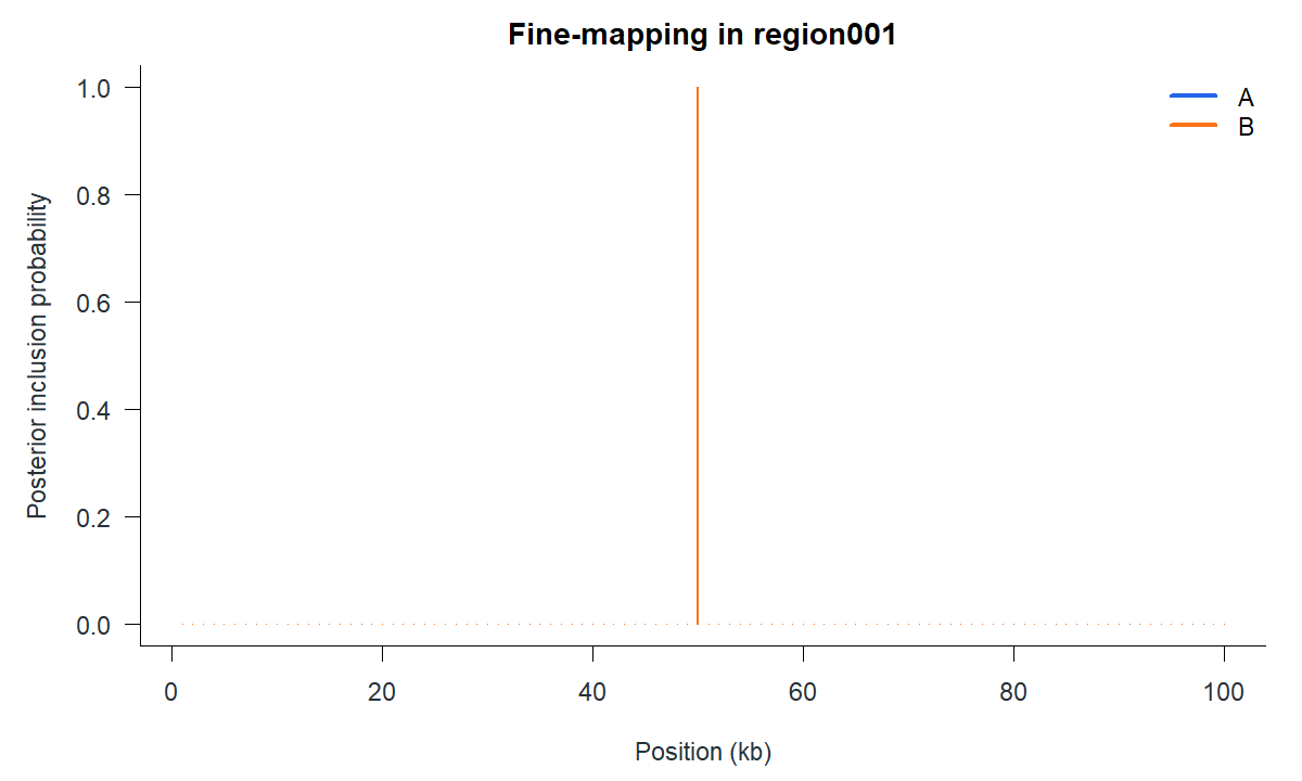
The plotted PIPs support m00050 for both traits under this one-effect model. Their high values are expected for the deliberately strong planted signal.
Check the numerical fit
Before interpreting a posterior set, inspect convergence, LD completeness, retained rank and fallback attempts. The first six region/trait rows from this run were accepted on the first attempt at full rank; no fallback was needed.
| Region | Trait | Status | Retained rank | Full rank | Requested retained positive mass | Achieved retained positive mass | Attempts | Fallback required |
|---|---|---|---|---|---|---|---|---|
| region001 | A | accepted | 100 | 100 | 0.995 | 1 | 1 | FALSE |
| region001 | B | accepted | 100 | 100 | 0.995 | 1 | 1 | FALSE |
| region002 | A | accepted | 100 | 100 | 0.995 | 1 | 1 | FALSE |
| region002 | B | accepted | 100 | 100 | 0.995 | 1 | 1 | FALSE |
| region003 | A | accepted | 100 | 100 | 0.995 | 1 | 1 | FALSE |
| region003 | B | accepted | 100 | 100 | 0.995 | 1 | 1 | FALSE |
subset(fit$diagnostic_summary,
  region %in% c("region001", "region002"))
subset(fit$eigen_attempts, region == "region001")
The full downloadable diagnostics include all 40 region/trait fits. A lower retained rank can change the likelihood, so the accepted threshold belongs in the reported result.
Summarize sets and Bayesian FDR
gmap_sets() returns ordinary set-level and marker-level data frames. The meaning of set mass depends on the fitted method; read the meaning column rather than treating every set as the same type of credible set.
posterior_sets <- gmap_sets(fit)
head(posterior_sets$summary)
head(posterior_sets$members)

fdr <- gmap_bfdr(fit, target = 0.05)
head(fdr[c("region", "trait", "selected_markers",
  "expected_false_discoveries", "bfdr")])
Bayesian FDR averages 1 - PIP among selected markers under the fitted posterior. It does not provide a frequentist FDR guarantee.
Compare traits and reuse saved fits
Component-pair colocalisation can use the saved multi-effect fits without refitting the regional models. The two simulated GWAS cohorts are disjoint; the complete 100-marker regions and reference are shared by both traits.
coloc <- gmap_coloc_components(fit, fit, reference_Glist,
  trait1 = "A", trait2 = "B", regions = "region001",
  control = list(complete_region_coverage = TRUE,
                 non_overlapping_samples = TRUE))
summary(coloc)
coloc$estimates
The colocalisation call illustrates a supported follow-on analysis; its probabilities were not included in the displayed run. Priors and eligibility checks are recorded in the returned result. For a global individual-level BayesC/BayesR fit, gmap_bed() instead groups its saved marker posterior within named regions using LD from the same fitted samples; those groups are not regional refits.